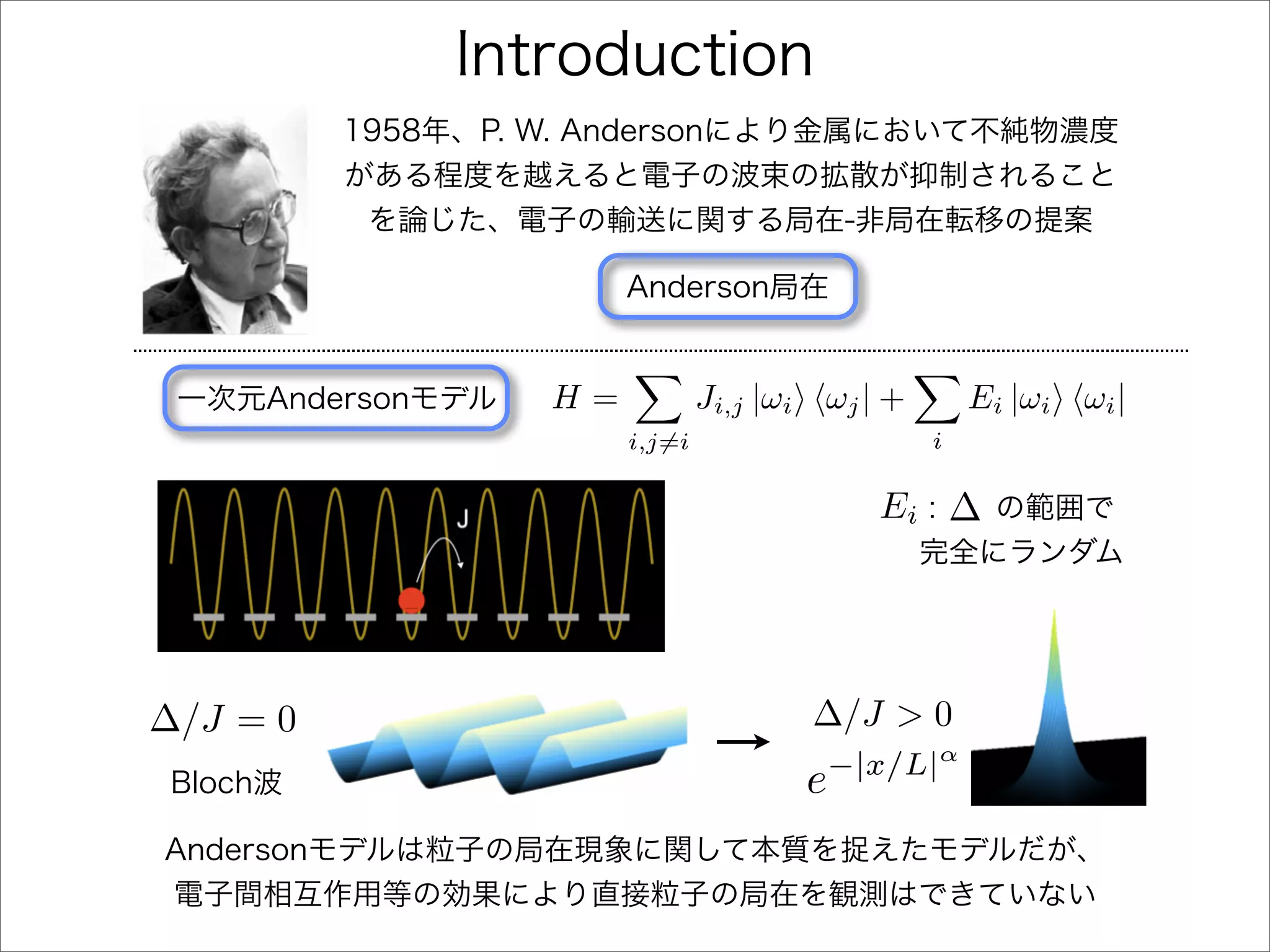
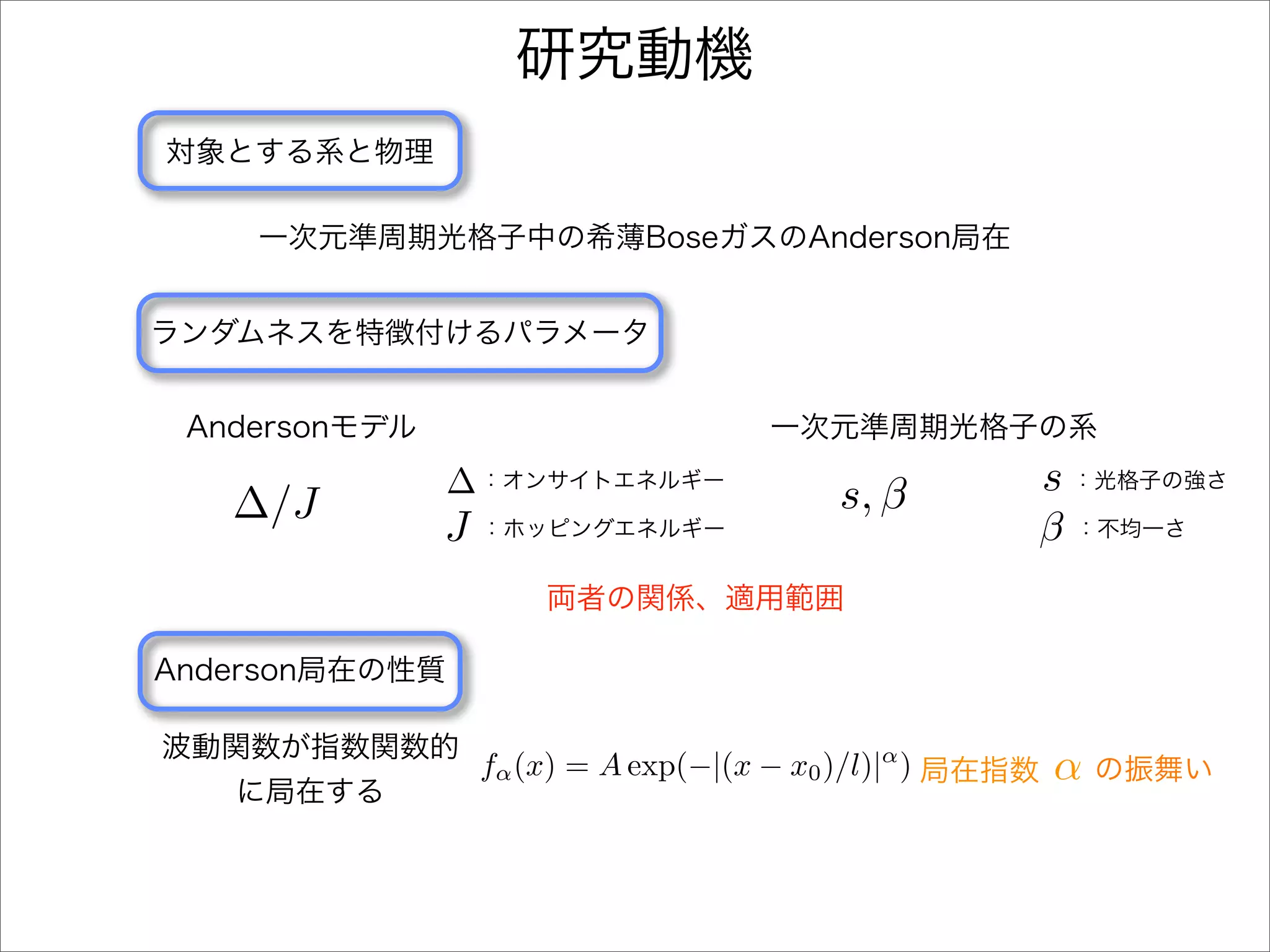
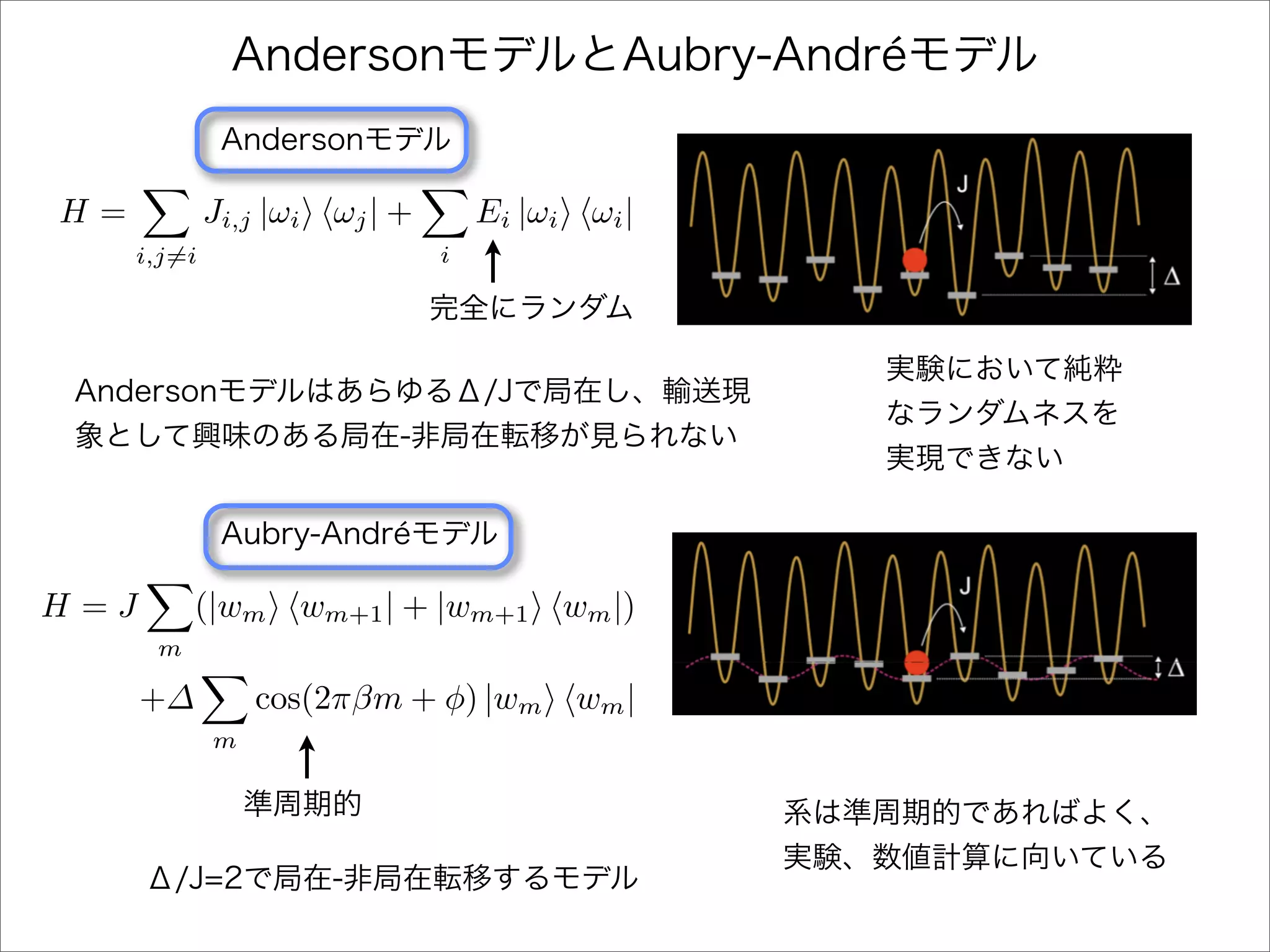
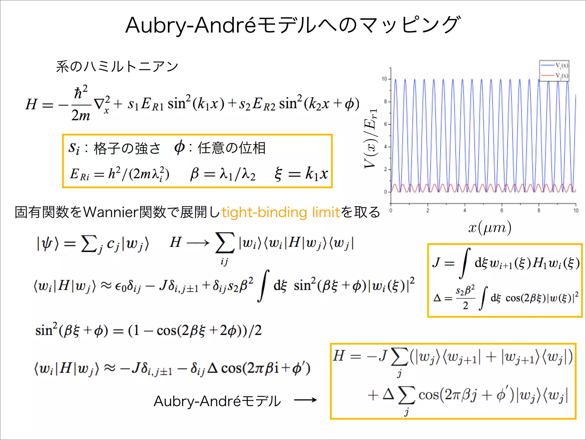
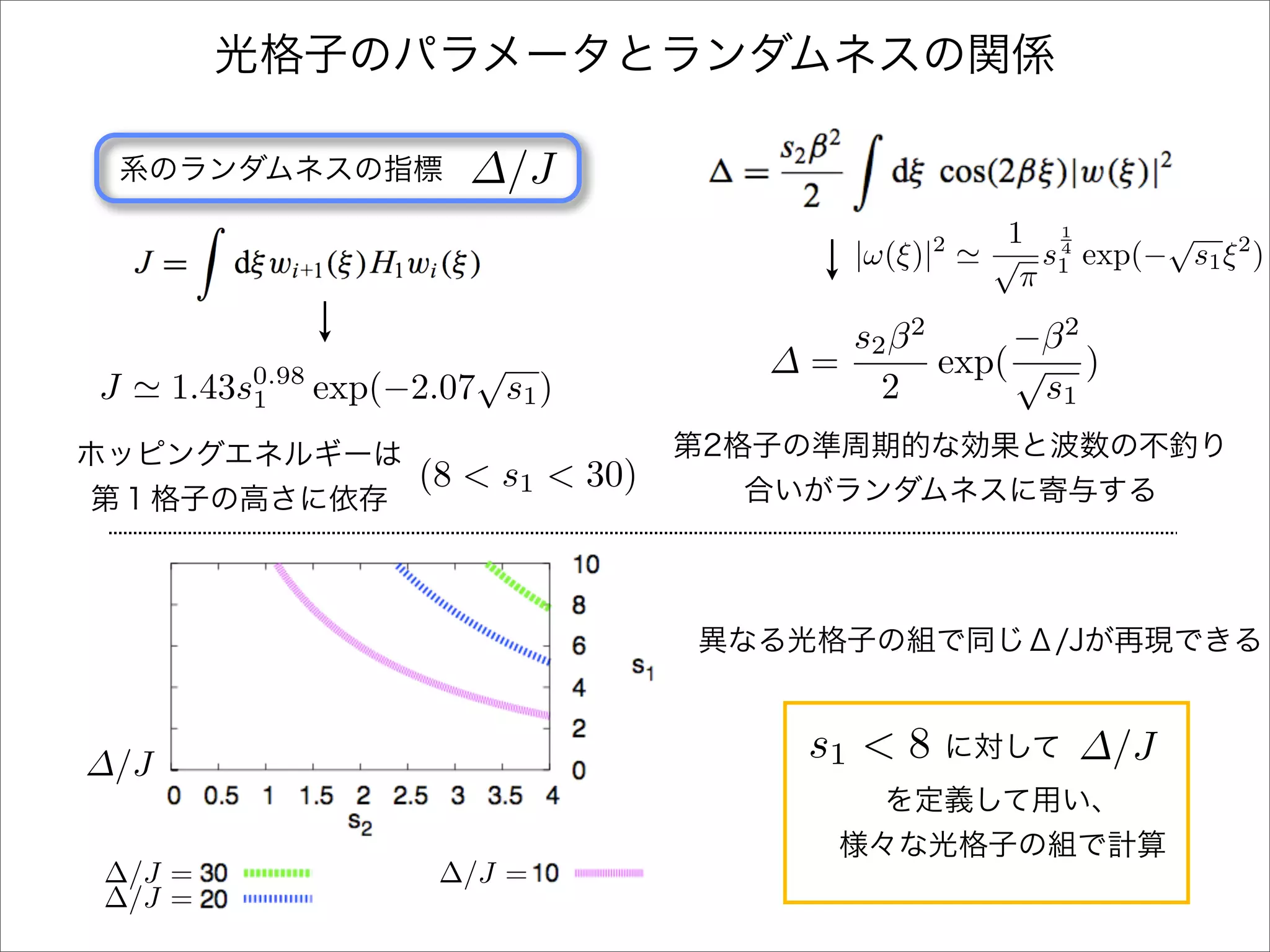
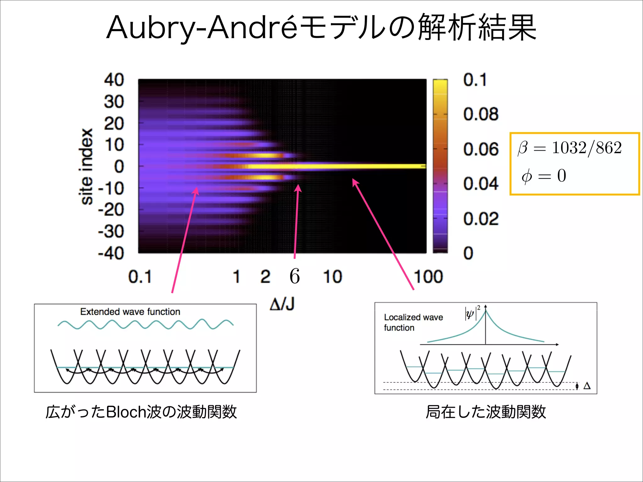
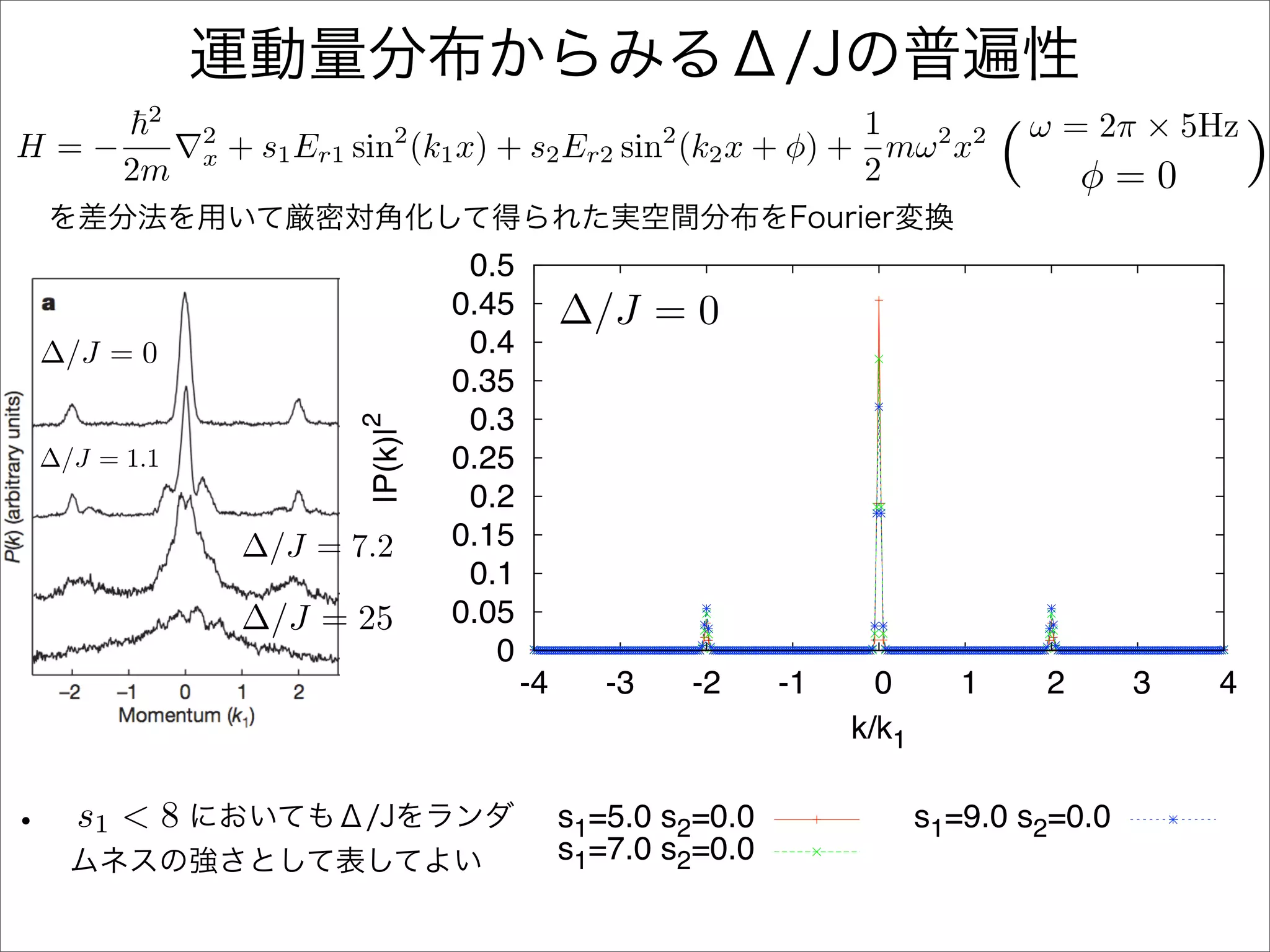
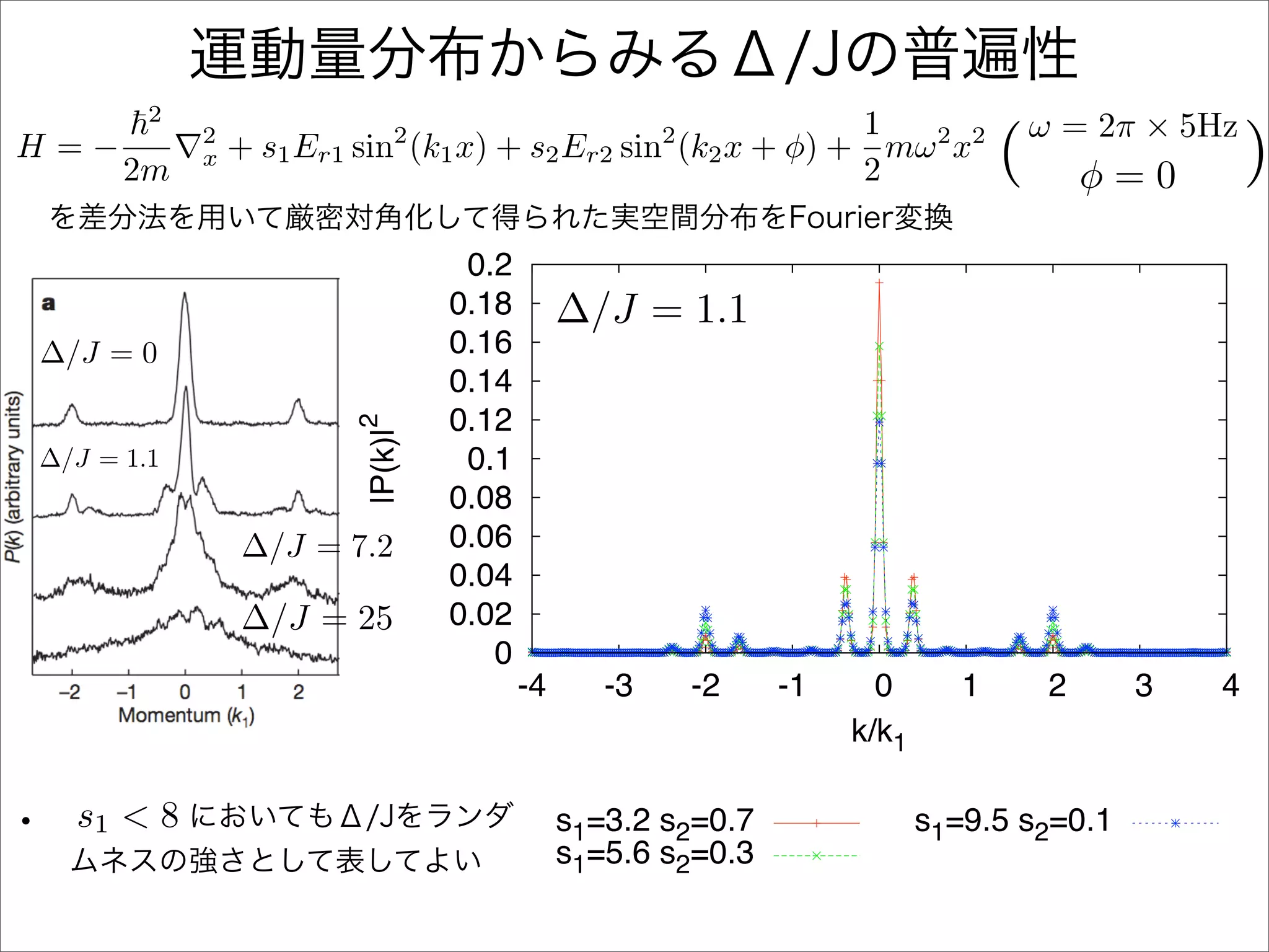
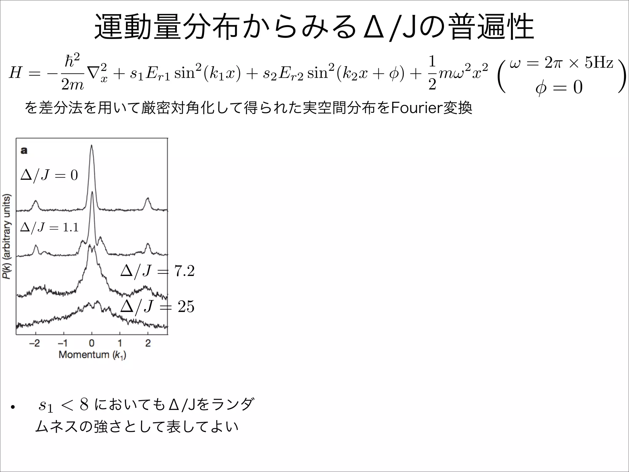
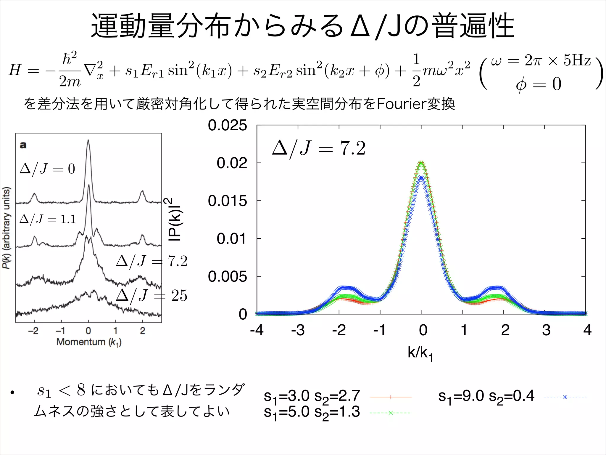
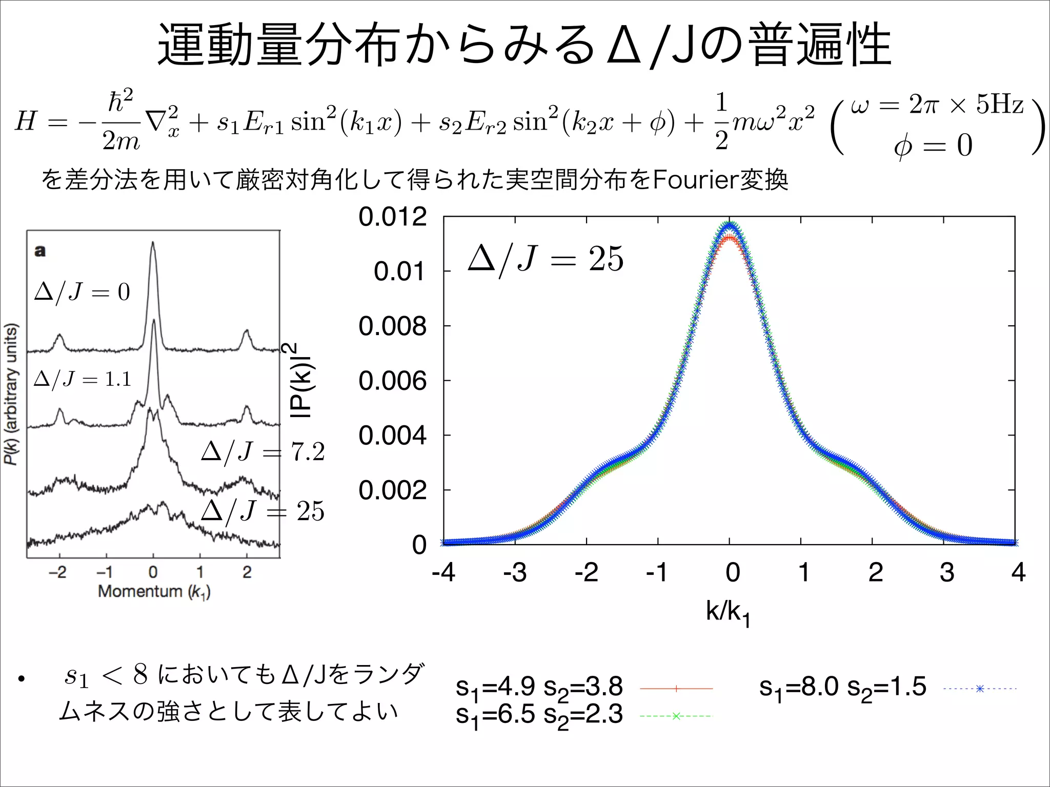
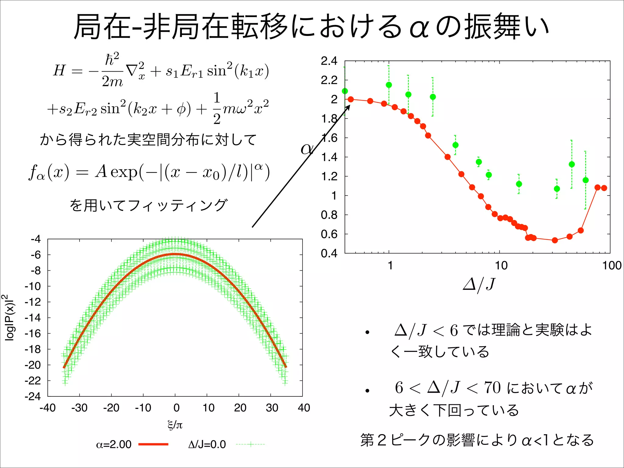
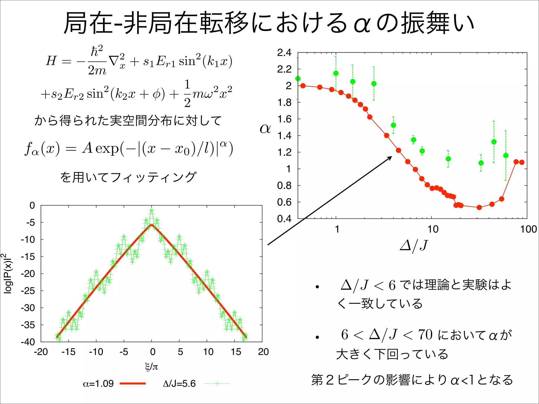
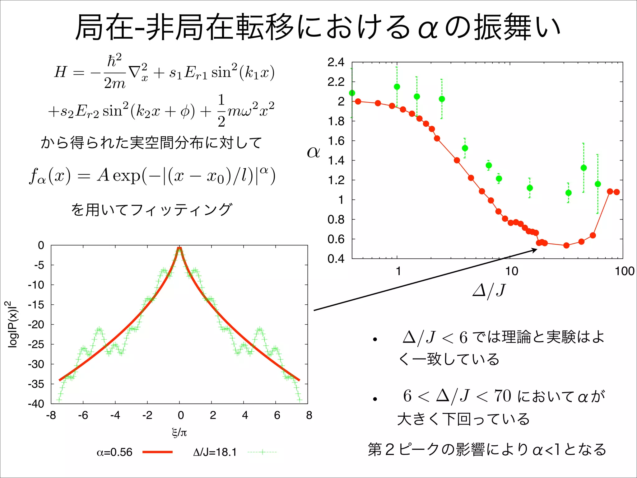
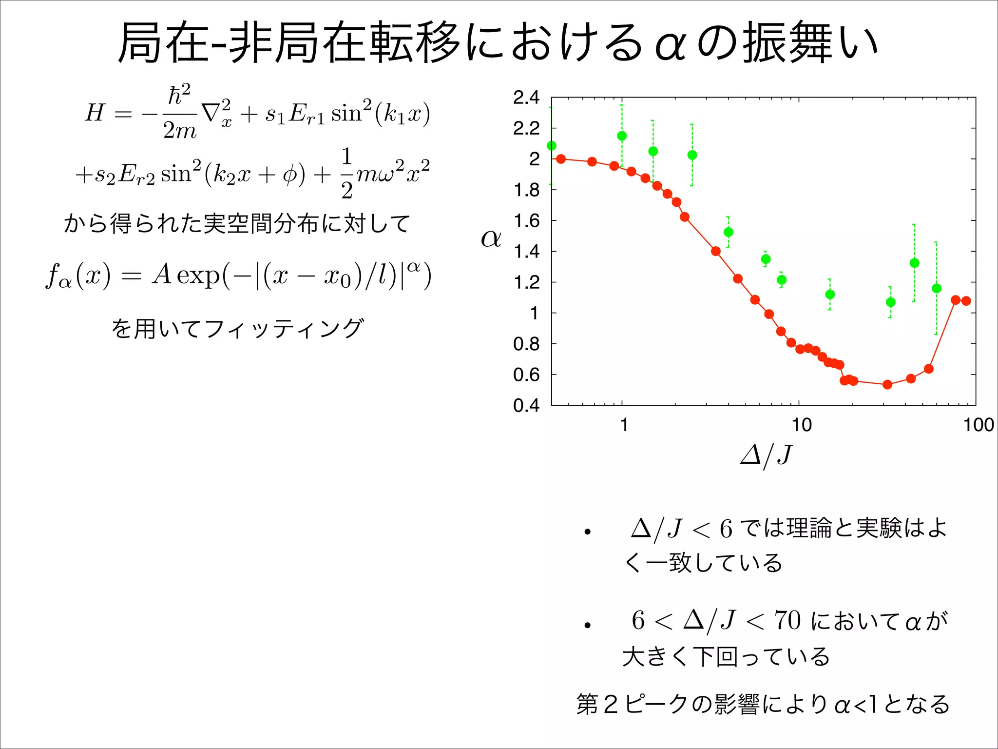
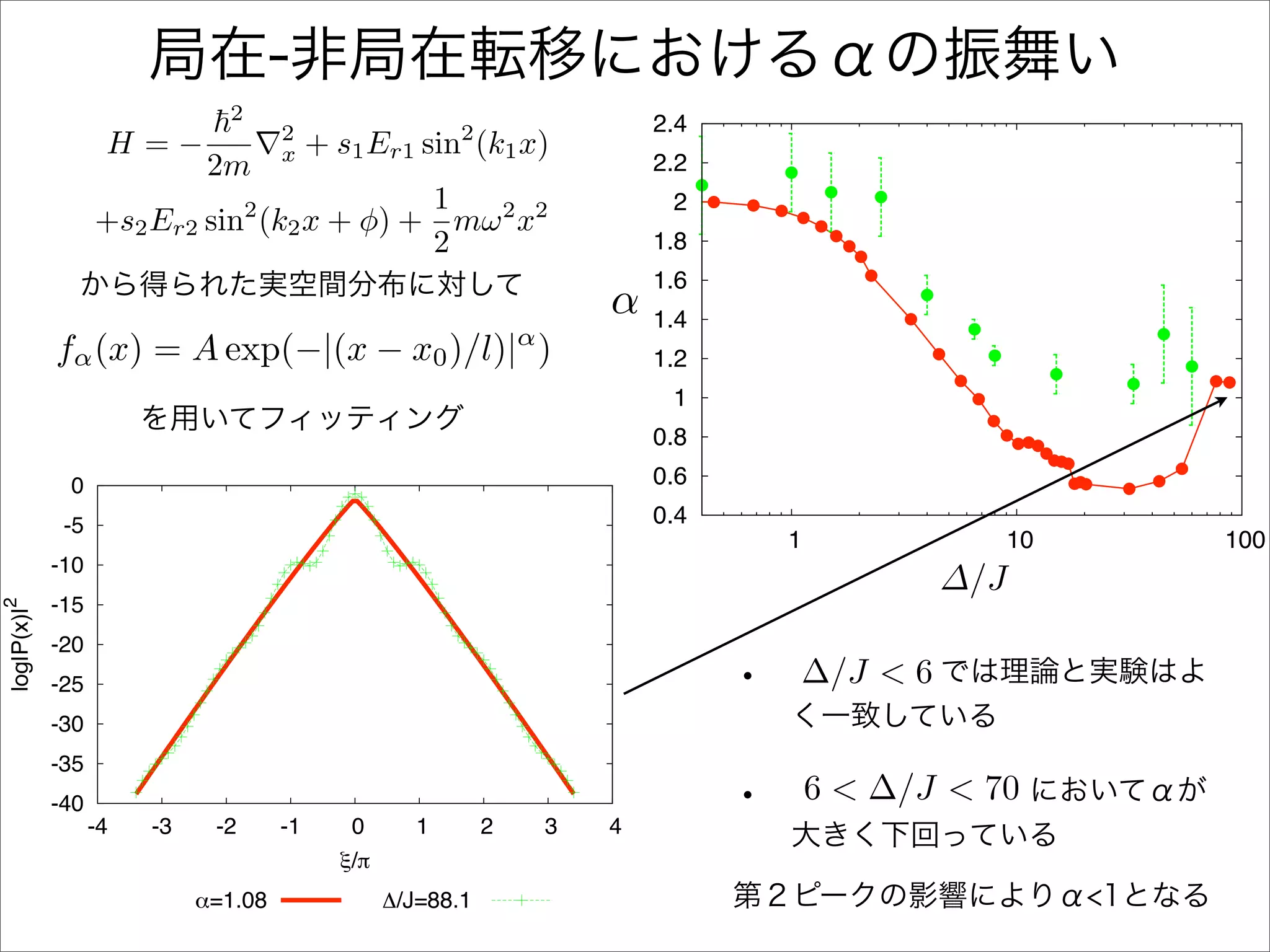
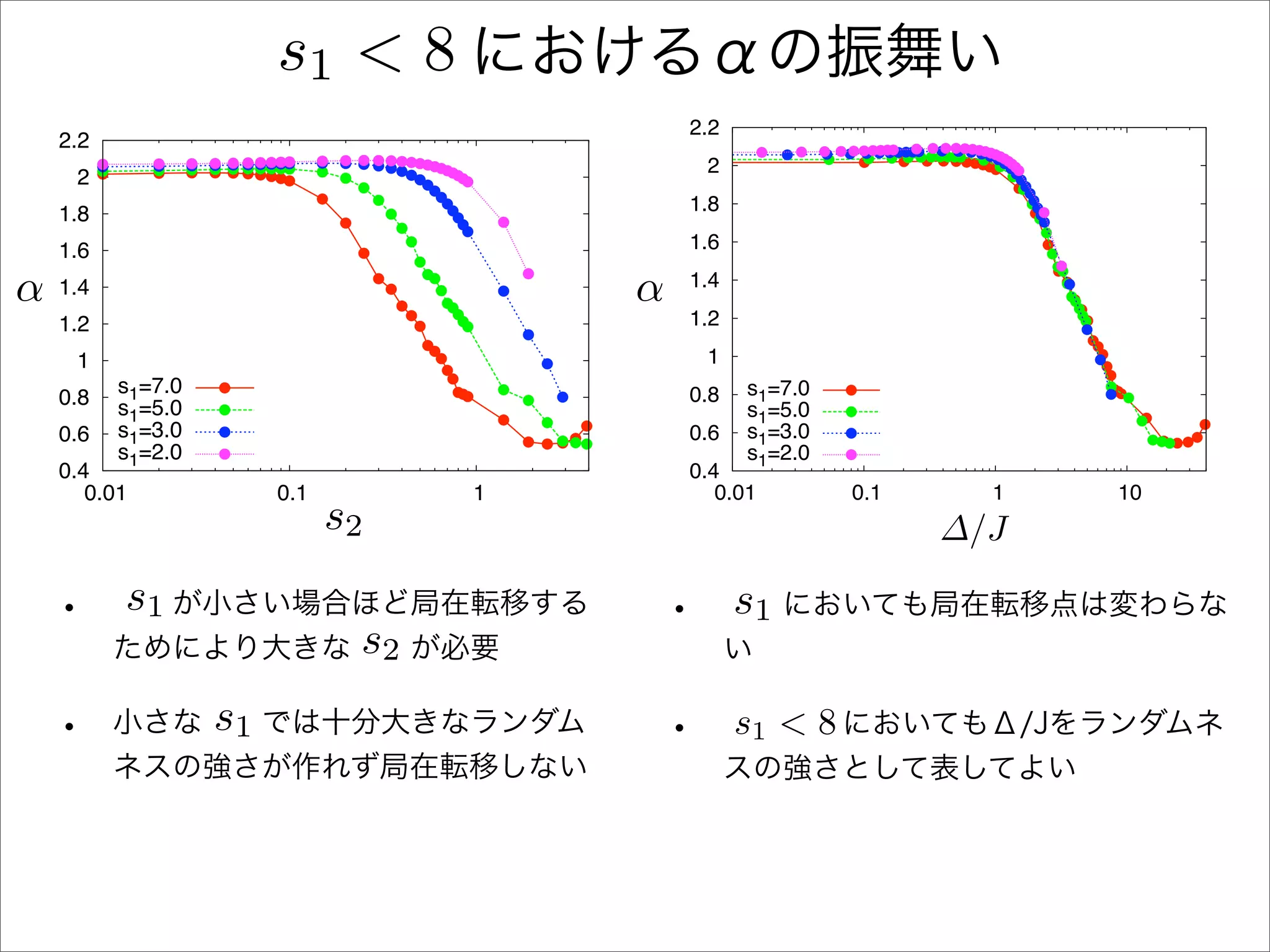
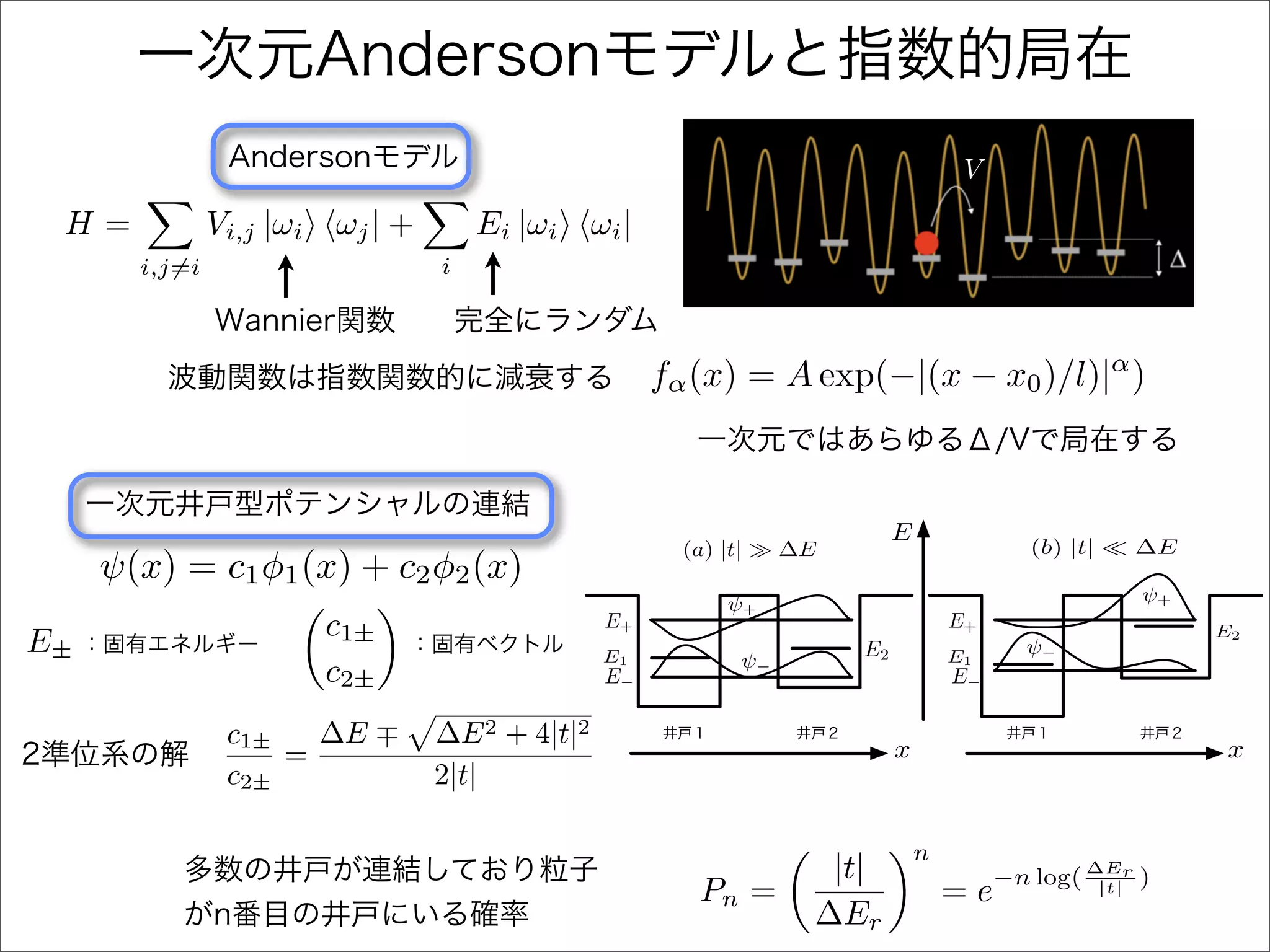
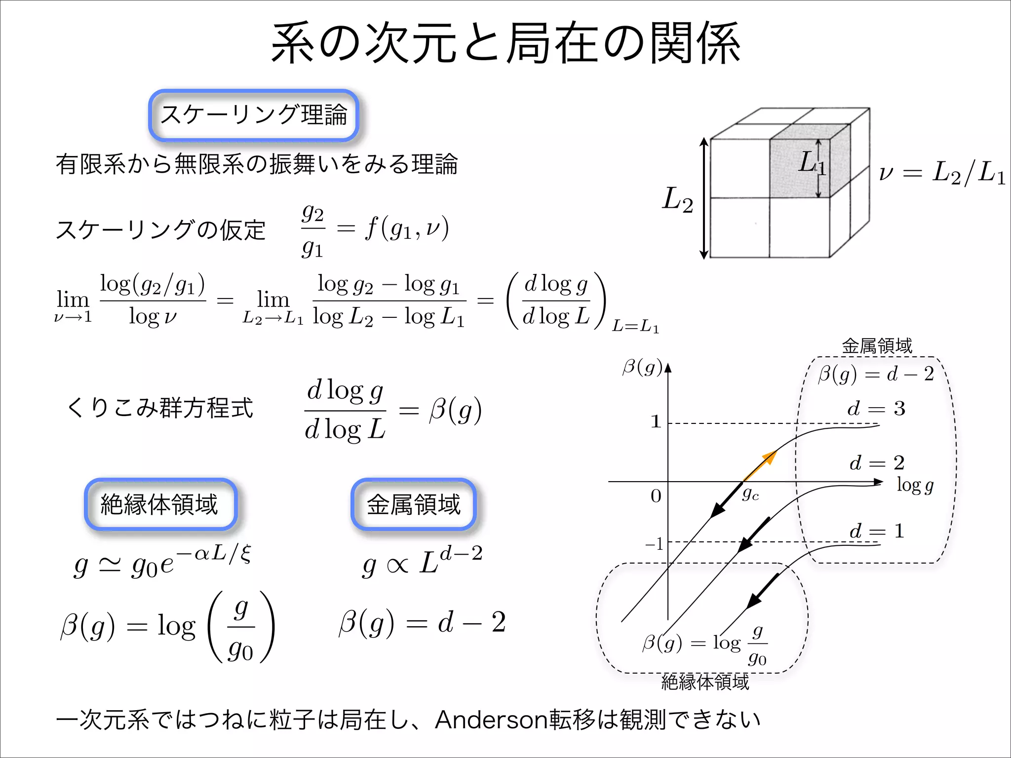
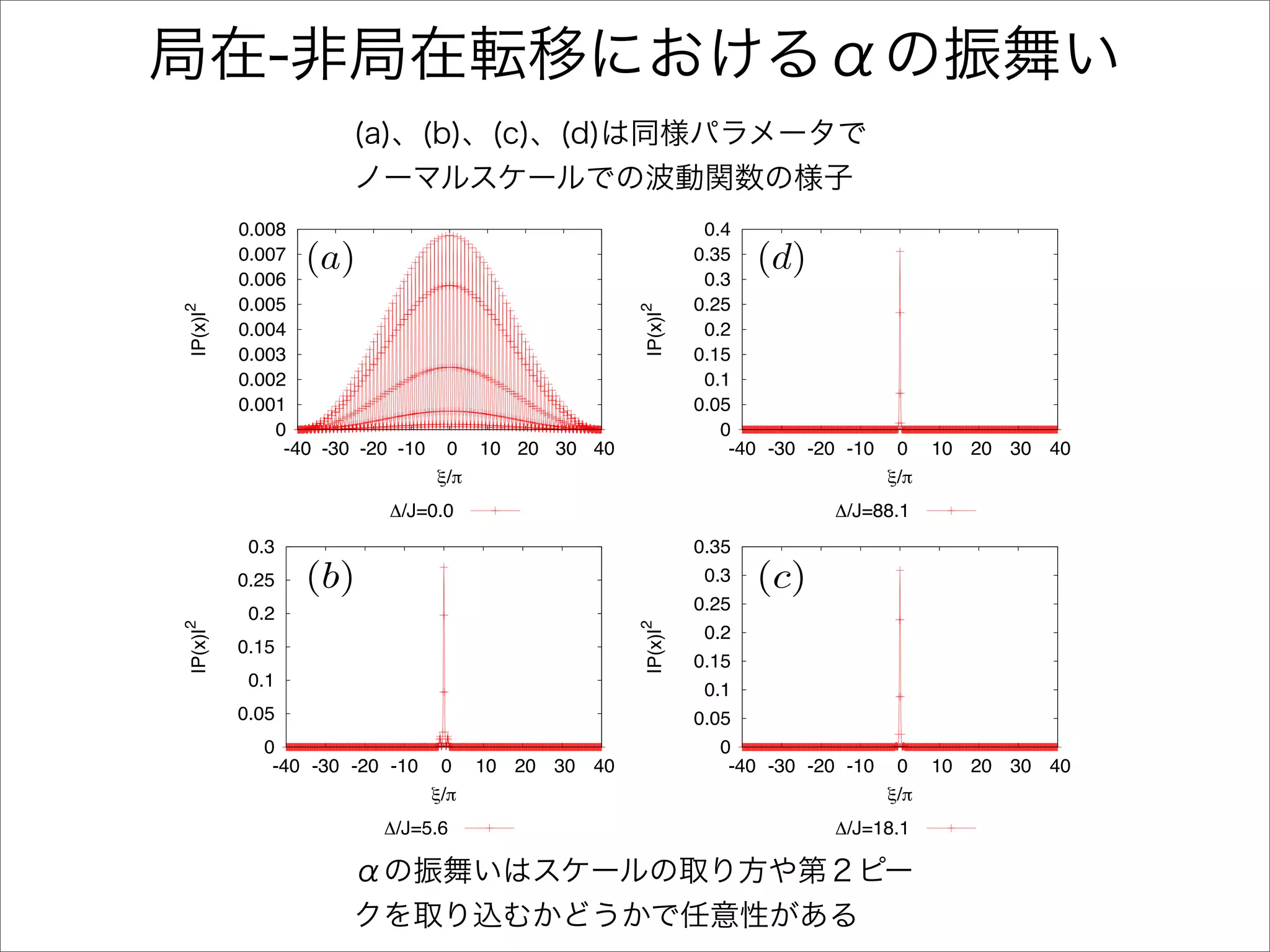
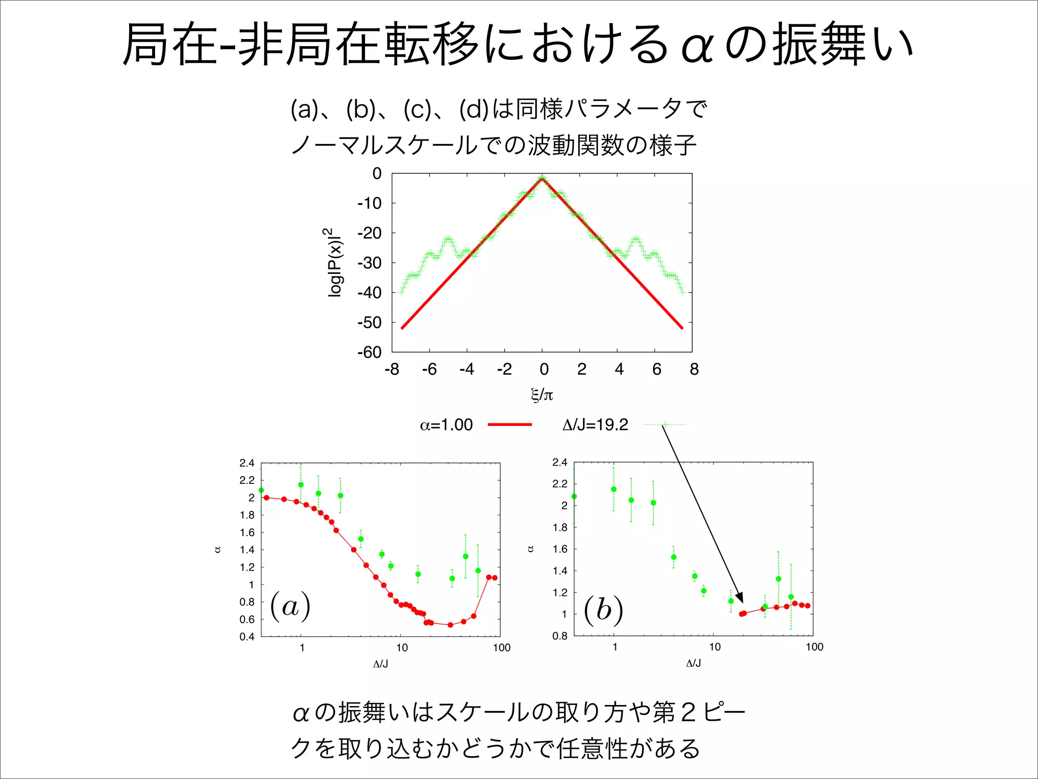
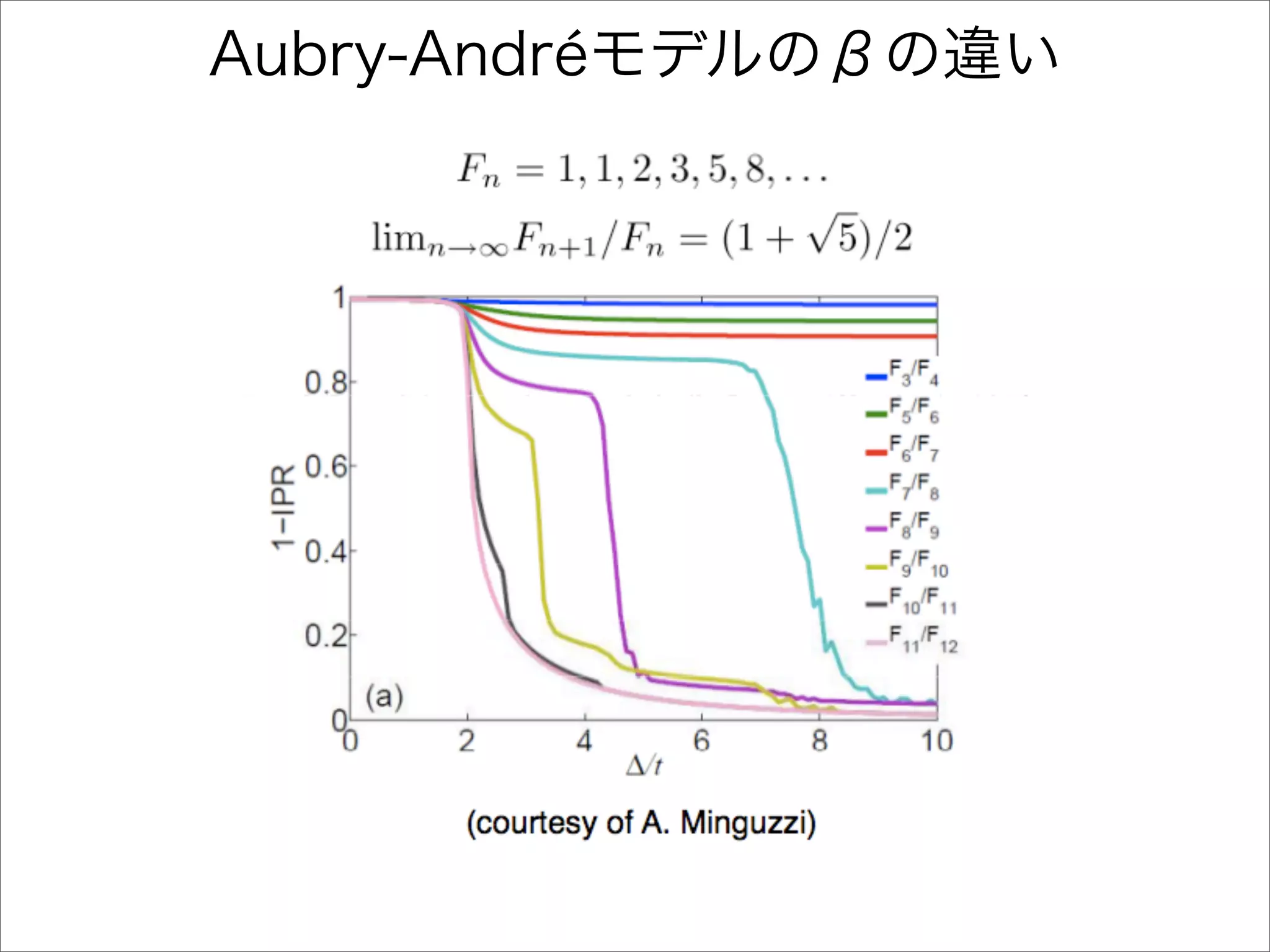
The document describes a Hamiltonian with terms including Ji,j|ωiωj| and Ei|ωiωi| that depends on parameters ∆/J and ω. It studies the behavior of the system as ∆/J increases from 0 to greater than 6, including plots of the momentum distribution |P(k)|2 that show it spreading out over more values of k/k1. The dependence of the system on other parameters like α, s1, and s2 is also examined through additional plots.

3. H= Ji,j |ωi ωj | + Ei |ωi ωi |
i,j=i i
Ei ∆
∆/J = 0 ∆/J > 0
−|x/L|α
e

4. H= Ji,j |ωi ωj | + Ei |ωi ωi |
i,j=i i
Ei ∆
∆/J = 0 ∆/J > 0
−|x/L|α
e

5. H= Ji,j |ωi ωj | + Ei |ωi ωi |
i,j=i i
T < Tc 1
N + U ni (ˆ i − 1)
ˆ n
ψ(r1 , r2 , · · · , rN , ) = φ0 (ri ) 2 i
i=1
V (x) = s1 Er1 sin2 (k1 x) + s2 Er2 sin2 (k2 x)
si i
β = k2 /k1
Ei

6. H= Ji,j |ωi ωj | + Ei |ωi ωi |
i,j=i i
T < Tc 1
N + U ni (ˆ i − 1)
ˆ n
ψ(r1 , r2 , · · · , rN , ) = φ0 (ri ) 2 i
i=1
V (x) = s1 Er1 sin2 (k1 x) + s2 Er2 sin2 (k2 x)
si i
β = k2 /k1
Ei

7. H= Ji,j |ωi ωj | + Ei |ωi ωi |
i,j=i i
T < Tc 1
N + U ni (ˆ i − 1)
ˆ n
ψ(r1 , r2 , · · · , rN , ) = φ0 (ri ) 2 i
i=1
V (x) = s1 Er1 sin2 (k1 x) + s2 Er2 sin2 (k2 x)
si i
β = k2 /k1
Ei
∆/J si , β

8. ∆ s
∆/J s, β
J β
fα (x) = A exp(−|(x − x0 )/l)|α ) α

10. H= Ji,j |ωi ωj | + Ei |ωi ωi |
i,j=i i
H=J (|wm wm+1 | + |wm+1 wm |)
m
+∆ cos(2πβm + φ) |wm wm |
m

11. V (x)/Er1
x(µm)

12. V (x)/Er1
x(µm)

13. V (x)/Er1
x(µm)

14. V (x)/Er1
x(µm)

15. ∆/J
1 1 √ 2
|ω(ξ)| 2
√ s1 exp(− s1 ξ )
4
π
s2 β 2 −β 2
√ ∆= exp( √ )
J 1.43s0.98
1 exp(−2.07 s1 ) 2 s1
(8 < s1 < 30)
∆/J
s1 < 8 ∆/J
∆/J = ∆/J =
∆/J =

17. European Laboratory for Non-Linear Spectroscopy (LENS)
39
K
1 1
Vho (x, r⊥ ) = mω x + mω⊥ r⊥
2 2 2 2
2 2
Energy
Position x(µm)

18. 0
1.8
∆/J
4.2
7
Time(ms) = 750
∆/J = 6
∆/J

19. ∆/J ≈ 1 ∆/J ≈ 15
fα (x) = A exp(−|(x − x0 )/l)|α )
Position x(µm)
α=2 α
α=1
∆/J

21. β = 1032/862
φ=0
6

22. 2
1 ω = 2π × 5Hz
H=−
2m
2
x + s1 Er1 sin (k1 x) + s2 Er2 sin (k2 x + φ) + mω 2 x2
2 2
2 ( φ=0 )
0.5
0.45 ∆/J = 0
∆/J = 0 0.4
0.35
0.3
|P(k)|2
∆/J = 1.1 0.25
0.2
∆/J = 7.2 0.15
0.1
∆/J = 25 0.05
0
-4 -3 -2 -1 0 1 2 3 4
k/k1
s1 < 8 s1=5.0 s2=0.0 s1=9.0 s2=0.0
s1=7.0 s2=0.0

23. 2
1 ω = 2π × 5Hz
H=−
2m
2
x + s1 Er1 sin (k1 x) + s2 Er2 sin (k2 x + φ) + mω 2 x2
2 2
2 ( φ=0 )
∆/J = 0
∆/J = 1.1
∆/J = 7.2
∆/J = 25
s1 < 8

24. 2
1 ω = 2π × 5Hz
H=−
2m
2
x + s1 Er1 sin (k1 x) + s2 Er2 sin (k2 x + φ) + mω 2 x2
2 2
2 ( φ=0 )
0.2
0.18 ∆/J = 1.1
∆/J = 0 0.16
0.14
0.12
|P(k)|2
∆/J = 1.1 0.1
0.08
∆/J = 7.2 0.06
0.04
∆/J = 25 0.02
0
-4 -3 -2 -1 0 1 2 3 4
k/k1
s1 < 8 s1=3.2 s2=0.7 s1=9.5 s2=0.1
s1=5.6 s2=0.3

25. 2
1 ω = 2π × 5Hz
H=−
2m
2
x + s1 Er1 sin (k1 x) + s2 Er2 sin (k2 x + φ) + mω 2 x2
2 2
2 ( φ=0 )
∆/J = 0
∆/J = 1.1
∆/J = 7.2
∆/J = 25
s1 < 8

26. 2
1 ω = 2π × 5Hz
H=−
2m
2
x + s1 Er1 sin (k1 x) + s2 Er2 sin (k2 x + φ) + mω 2 x2
2 2
2 ( φ=0 )
0.025
∆/J = 7.2
∆/J = 0 0.02
0.015
2
|P(k)|
∆/J = 1.1
0.01
∆/J = 7.2
0.005
∆/J = 25
0
-4 -3 -2 -1 0 1 2 3 4
k/k1
s1 < 8 s1=3.0 s2=2.7 s1=9.0 s2=0.4
s1=5.0 s2=1.3

27. 2
1 ω = 2π × 5Hz
H=−
2m
2
x + s1 Er1 sin (k1 x) + s2 Er2 sin (k2 x + φ) + mω 2 x2
2 2
2 ( φ=0 )
∆/J = 0
∆/J = 1.1
∆/J = 7.2
∆/J = 25
s1 < 8

28. 2
1 ω = 2π × 5Hz
H=−
2m
2
x + s1 Er1 sin (k1 x) + s2 Er2 sin (k2 x + φ) + mω 2 x2
2 2
2 ( φ=0 )
0.012
0.01 ∆/J = 25
∆/J = 0
0.008
|P(k)|2
∆/J = 1.1 0.006
0.004
∆/J = 7.2
0.002
∆/J = 25
0
-4 -3 -2 -1 0 1 2 3 4
k/k1
s1 < 8 s1=4.9 s2=3.8 s1=8.0 s2=1.5
s1=6.5 s2=2.3

29. 2
2.4
H=− 2
+ s1 Er1 sin (k1 x)
2
2m x 2.2
1 2
+s2 Er2 sin (k2 x + φ) + mω 2 x2
2
2 1.8
1.6
α 1.4
!
fα (x) = A exp(−|(x − x0 )/l)| ) α
1.2
1
0.8
-4 0.6
-6 0.4
-8 1 10 100
-10 ∆/J
"/J
log|P(x)|2
-12
-14
-16 ∆/J < 6
-18
-20
-22
-24
6 < ∆/J < 70
-40 -30 -20 -10 0 10 20 30 40
!/"
#=2.00 $/J=0.0

30. 2
2.4
H=− 2
+ s1 Er1 sin (k1 x)
2
2m x 2.2
1 2
+s2 Er2 sin (k2 x + φ) + mω 2 x2
2
2 1.8
1.6
α 1.4
!
fα (x) = A exp(−|(x − x0 )/l)| ) α
1.2
1
0.8
0.6
0.4
1 10 100
∆/J
"/J
∆/J < 6
6 < ∆/J < 70

31. 2
2.4
H=− 2
+ s1 Er1 sin (k1 x)
2
2m x 2.2
1 2
+s2 Er2 sin (k2 x + φ) + mω 2 x2
2
2 1.8
1.6
α 1.4
!
fα (x) = A exp(−|(x − x0 )/l)| ) α
1.2
1
0.8
0 0.6
-5 0.4
1 10 100
-10
∆/J
"/J
-15
log|P(x)|2
-20
-25 ∆/J < 6
-30
-35
-40
6 < ∆/J < 70
-20 -15 -10 -5 0 5 10 15 20
!/"
#=1.09 $/J=5.6

32. 2
2.4
H=− 2
+ s1 Er1 sin (k1 x)
2
2m x 2.2
1 2
+s2 Er2 sin (k2 x + φ) + mω 2 x2
2
2 1.8
1.6
α 1.4
!
fα (x) = A exp(−|(x − x0 )/l)| ) α
1.2
1
0.8
0.6
0.4
1 10 100
∆/J
"/J
∆/J < 6
6 < ∆/J < 70

33. 2
2.4
H=− 2
+ s1 Er1 sin (k1 x)
2
2m x 2.2
1 2
+s2 Er2 sin (k2 x + φ) + mω 2 x2
2
2 1.8
1.6
α 1.4
!
fα (x) = A exp(−|(x − x0 )/l)| ) α
1.2
1
0.8
0
0.6
-5
0.4
1 10 100
-10
∆/J
"/J
-15
log|P(x)|2
-20
-25 ∆/J < 6
-30
-35
-40
6 < ∆/J < 70
-8 -6 -4 -2 0 2 4 6 8
!/"
#=0.56 $/J=18.1

34. 2
2.4
H=− 2
+ s1 Er1 sin (k1 x)
2
2m x 2.2
1 2
+s2 Er2 sin (k2 x + φ) + mω 2 x2
2
2 1.8
1.6
α 1.4
!
fα (x) = A exp(−|(x − x0 )/l)| ) α
1.2
1
0.8
0.6
0.4
1 10 100
∆/J
"/J
∆/J < 6
6 < ∆/J < 70

35. 2
2.4
H=− 2
+ s1 Er1 sin (k1 x)
2
2m x 2.2
1 2
+s2 Er2 sin (k2 x + φ) + mω 2 x2
2
2 1.8
1.6
α 1.4
!
fα (x) = A exp(−|(x − x0 )/l)| ) α
1.2
1
0.8
0 0.6
-5 0.4
1 10 100
-10
∆/J
"/J
-15
log|P(x)|2
-20
-25 ∆/J < 6
-30
-35
-40
6 < ∆/J < 70
-4 -3 -2 -1 0 1 2 3 4
!/"
#=1.08 $/J=88.1

36. s1 < 8
2.2
2.2
2
2
1.8 1.8
1.6 1.6
α 1.4 α 1.4
!
!
1.2 1.2
1 1
s1=7.0 0.8 s1=7.0
0.8 s1=5.0 s1=5.0
0.6 s1=3.0 0.6 s1=3.0
s1=2.0 s1=2.0
0.4 0.4
0.01 0.1 1 0.01 0.1 1 10
s2
s
2 ∆/J
"/J
s1 s1
s2
s1 s1 < 8

37. s1 < 8
∆/J

38. V
H= Vi,j |ωi ωj | + Ei |ωi ωi |
i,j=i i
fα (x) = A exp(−|(x − x0 )/l)|α )
E
(a) |t| ∆E (b) |t| ∆E
ψ(x) = c1 φ1 (x) + c2 φ2 (x)
ψ+ ψ+
E± c1± E+ E+ E2
E1 E2 E1 ψ−
ψ−
c2± E− E−
c1± ∆E ∆E 2 + 4|t|2
= x x
c2± 2|t|
n
|t| −n log( ∆Er )
Pn = =e |t|
∆Er

39. L1 ν = L2 /L1
g2 L2
= f (g1 , ν)
g1
log(g2 /g1 ) log g2 − log g1 d log g
lim = lim =
ν→1 log ν L2 →L1 log L2 − log L1 d log L L=L1
β(g) β(g) = d − 2
d log g
= β(g) 1
d=3
d log L
d=2
gc log g
0
d=1
−1
g g0 e−αL/ξ g ∝ Ld−2
g
β(g) = log β(g) = d − 2 g
g0 β(g) = log
g0

40. )#
!"#""+ !"#(
!"#""*
!"#"")
(a) !(# !"#'$
!"#'
(d)
!'#
+,-./012.'
!"#""( !"#&$
-./01-%
&
*+,-.*
!"#""' !&# !"#&
!"#""& !%# !"#%$
!"#""% !"#%
!"#""$
!$# !"#"$
!" !"# !"
,'" ,&" ,%" ,$" !" !* !%" !&" !'"
!$" !" !% !' )# )' )(" )'")")&" )*
)% )%" !" !%" !&" !'" !("
!2" !3" !/"
#234"#"! #4(5##) $364(75') #/0122#%!
!"#' !"#'$
(b) (c)
!(#$ !&#'
!"#&$ !"#'
!(#( !&#&
!( !"#&$
!"#& !&
*+,-.*&
*+,-.*&
!'#& !"#&
!"#%$ !'#% !%#$
!'#$
!"#%$
!%#(
!
!
!"#%
!'#( !%#' !"#%
!"#"$ !' !"#"$
(a)
!%#&
!"#&
!" !"#%
()" ('" (&" (%" !" !%" !&" !'" !)"
!% (b) ('"
!"
()" (&" (%" !" !%" !&" !'" !)"
!"#$ !"#$
!' !/" !'" !'"" !% !%" !/" !%""
")* ")*
#/01$#2! #/01%2#%!

41. )#
!(#
!'#
+,-./012.'
!&#
!%#
!$#
!"#
!* !" !% !' )# )' )% )" )*
!3"
#4(5##) $364(75')
!(#$ !&#'
!(#( !&#&
!(
!&
!'#&
!'#% !%#$
!'#$ !%#(
!
!
!'#( !%#'
!'
(a)
!%#&
!"#&
!"#% !% (b)
!"#$ !"#$
!' !'" !'"" !% !%" !%""
")* ")*

43. ( < x >2 )[µm]
!'"
)$*$"(+
!&# )$*,('
)$*#(+
!&"
!%#
√
!%"
!$#
!$"
!#
!"
!"#
!"("$ !"($ !$
)%
s2
!'"
)$*$"(+
!&# )$*,('
)$*#(+
!&"
!%#
>
!%"
x2
<
!$#
s1
√
!$"
!#
!"
!"("$ !"($ !$
)%