The document outlines research on developing optimal finite difference grids for solving elliptic and parabolic partial differential equations (PDEs). It introduces the motivation to accurately compute Neumann-to-Dirichlet (NtD) maps. It then summarizes the formulation and discretization of model elliptic and parabolic PDE problems, including deriving the discrete NtD map. It presents results on optimal grid design and the spectral accuracy achieved. Future work is proposed on extending the NtD map approach to non-uniformly spaced boundary data.

1. Introduction Elliptic problem Parabolic problem Proposed Work Conclusion
Optimal Finite Difference Grids for Elliptic and
Parabolic PDEs with Applications
Oleksiy Varfolomiyev
Advisor Prof. Michael Siegel
Co-Advisor Prof. Michael Booty
NJIT, May 15, 2012

2. Introduction Elliptic problem Parabolic problem Proposed Work Conclusion
Outline
1 Introduction
Motivation
2 Elliptic problem
Problem Formulation
Discretization and NtD map
Approximation Error
Grids and Numerical Results
NtD map for nonuniformly spaced boundary data
3 Parabolic problem
Problem Formulation
Discretization
Benchmarks
4 Proposed Work
5 Conclusion

3. Introduction Elliptic problem Parabolic problem Proposed Work Conclusion
Motivation
Motivation
Problem
Accurate and efficient computation of the DtN (NtD) maps
Applications of interest
1 Water waves: DtN map is used to compute the normal
interface speed
2 Crystal growth: DtN map is used to track the crystal-melt
interface
3 Surface with soluble surfactant: DtN map is used to resolve
surfactant concentration gradient

4. Introduction Elliptic problem Parabolic problem Proposed Work Conclusion
Elliptic Problem

5. Introduction Elliptic problem Parabolic problem Proposed Work Conclusion
Problem Formulation
1
Model Elliptic Problem Formulation
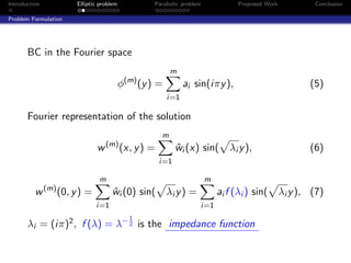
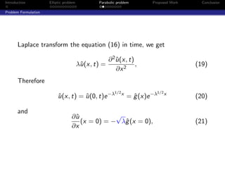
Laplace equation on a semi-infinite strip
∂ 2 w (x, y ) ∂ 2 w (x, y )
− − = 0, (x, y ) ∈ [0, ∞) × [0, 1], (1)
∂y 2 ∂x 2
∂w
(0, y ) = −ϕ(y ), y ∈ [0, 1], (2)
∂x
w |x=∞ = 0, (3)
w (x, 0) = 0, w (x, 1) = 0, x ∈ [0, ∞). (4)
1
V. Druskin

6. Introduction Elliptic problem Parabolic problem Proposed Work Conclusion
Problem Formulation
1
Model Elliptic Problem Formulation
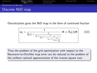
Laplace equation on a semi-infinite strip
∂ 2 w (x, y ) ∂ 2 w (x, y )
− − = 0, (x, y ) ∈ [0, ∞) × [0, 1], (1)
∂y 2 ∂x 2
∂w
(0, y ) = −ϕ(y ), y ∈ [0, 1], (2)
∂x
w |x=∞ = 0, (3)
w (x, 0) = 0, w (x, 1) = 0, x ∈ [0, ∞). (4)
Our goal is to accurately resolve the Dirichlet data w (0, y )
1
V. Druskin

7. Introduction Elliptic problem Parabolic problem Proposed Work Conclusion
Problem Formulation
BC in the Fourier space
m
φ(m) (y ) = ai sin(iπy ), (5)
i=1
Fourier representation of the solution
m
w (m) (x, y ) = wi (x) sin(
ˆ λi y ), (6)
i=1

8. Introduction Elliptic problem Parabolic problem Proposed Work Conclusion
Problem Formulation
BC in the Fourier space
m
φ(m) (y ) = ai sin(iπy ), (5)
i=1
Fourier representation of the solution
m
w (m) (x, y ) = wi (x) sin(
ˆ λi y ), (6)
i=1
m m
(m)
w (0, y ) = wi (0) sin(
ˆ λi y ) = ai f (λi ) sin( λi y ), (7)
i=1 i=1
1
λi = (iπ)2 , f (λ) = λ− 2 is the impedance function

9. Introduction Elliptic problem Parabolic problem Proposed Work Conclusion
Discretization and NtD map
Discretization
Fourier transform (1) in y
∂ 2 wk (x)
ˆ
λk wk (x) −
ˆ = 0, k = 1, . . . , m (8)
∂x 2
∂ wk (0)
ˆ
= −ϕk ,
ˆ k = 1, . . . , m, (9)
∂x
where λk = (kπ)2 .

10. Introduction Elliptic problem Parabolic problem Proposed Work Conclusion
Discretization and NtD map
Discretization
Fourier transform (1) in y
∂ 2 wk (x)
ˆ
λk wk (x) −
ˆ = 0, k = 1, . . . , m (8)
∂x 2
∂ wk (0)
ˆ
= −ϕk ,
ˆ k = 1, . . . , m, (9)
∂x
where λk = (kπ)2 .
Discretize in x
1 wi+1 − wi wi − wi−1
λwi − − = 0, i = 2, . . . , n, (10)
ˆi
h hi hi−1
1 w2 − w1 1 w1 − w0
λw1 − =− = Φ (11)
ˆ1
h h1 ˆ1
h h0
where wi = wk (xi ), Φ = ϕk , (w1 − w0 )/h0 is set to Φ and λ = λk .
ˆ ˆ

11. Introduction Elliptic problem Parabolic problem Proposed Work Conclusion
Discretization and NtD map
Discrete NtD map
Discretization gives the NtD map in the form of continued fraction
1
w1 = Φ ≡ Rn (λ)Φ (12)
ˆ
h1 λ + 1
1
h1 + ˆ 1
h2 λ+···+ 1
hn−1 +
hn λ+ 1
ˆ
hn
Thus the problem of the grid optimization with respect to the
Neumann-to-Dirichlet map error can be reduced to the problem of
the uniform rational approximation of the inverse square root.

12. Introduction Elliptic problem Parabolic problem Proposed Work Conclusion
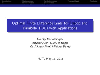
Discretization and NtD map
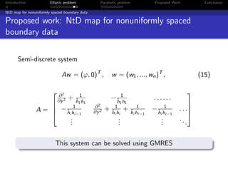
F - Fourier transform in y , F −1 - inverse Fourier transform in y
NtD Map
∂w
Given Neumann data ∂x (0, y ) = −ϕ(y ), y ∈ [0, 1]
w1 = F −1 Rn F ϕ, (13)
DtN Map
Given Dirichlet data w (0, y ) = ψ(y ), y ∈ [0, 1]
φ = −F −1 Rn F ψ
−1
(14)

13. Introduction Elliptic problem Parabolic problem Proposed Work Conclusion
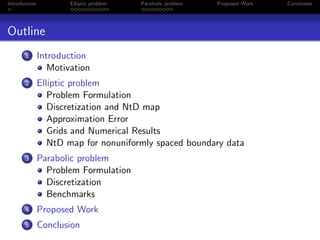
Approximation Error
Approximation Error
L2 error of the semidiscrete solution at x = 0
(n) 1
en = ||w (m) (0, y ) − w1 (y )||L2 [0,1] ≤ ||ϕ||L2 [0,1] max |fn (λ) − λ− 2 |
λ∈[π 2 ,(mπ)2 ]
1
π2 n
En (λ) = maxλ∈[λmin ,λmax ] fn (λ) − λ− 2 = O exp λ
log λ min
max
The described special choice of the discretization grid steps
provides a spectral convergence order of the solution at the
boundary.

14. Introduction Elliptic problem Parabolic problem Proposed Work Conclusion
Approximation Error
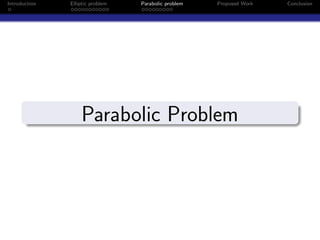
Relative Error Plot
Pk (λ)−λ−1/2
Relative error E (λ) = λ−1/2
0.01
4
4
10
10
6
10
7
10
relative error
8
10
10
10
10
10
13
10 12
10
14
10
0.1 1 10 100 1000 104 105
Λ 1 10 100 1000 104
Figure: Relative Error in the approximation of the inverse square root,
k = 16, λ ∈ [1, 10000] (left), λ ∈ [1, 1000] (right)

15. Introduction Elliptic problem Parabolic problem Proposed Work Conclusion
Grids and Numerical Results
Optimal geometric grids 0
10
fk(λ) − λ−1/2
−2
10
−4
10
√ √ −6
π/ k
h1 = e − kπ 10
α=e
error
√ −8
10
i−1 π(i−k−1)/ k
hi = h1 α =e −10
10
√
ˆ
h1 = h1 /(1 + α) −12
10
ˆ
−14
10
hi = hi hi−1 10
0
10
1
10
2
10
3
frequency
10
4
10
5
10
6 7
10
fk(λ) − λ−1/2
−3
10
−4
10
Nonoptimal geometric grids
−5
error 10
−6
10
ˆ hy
h1 = O(hy ) h1 = √ 10
−7
1+ α
−8
10
0 1 2 3 4 5 6 7
10 10 10 10 10 10 10 10
frequency

16. Introduction Elliptic problem Parabolic problem Proposed Work Conclusion
Grids and Numerical Results
Numerical Results
We discretize second derivatives in y using a second order,
centered finite difference scheme. The resulting system matrix is
sparse-banded.
Example with Neumann data ϕ(y ) = sin(πy )
−11 Abs. error in approximation of Dir BC
x 10 x 10
−4 Abs. error in approximation of Dir BC Abs. error for node x2
1.4 0.5
0.035
1.2 0
0.03
−0.5
1
0.025
−1
0.8
−1.5 0.02
0.6 −2
0.015
−2.5
0.4 0.01
−3
0.2 0.005
−3.5
(a) 0
0 0.1 0.2 0.3 0.4 0.5 0.6 0.7 0.8 0.9 1 (b) −4
0 0.1 0.2 0.3 0.4 0.5 0.6 0.7 0.8 0.9 1 (c) 0
0 0.1 0.2 0.3 0.4 0.5 0.6 0.7 0.8 0.9 1
Figure: (a) Error E (y ) = |w (0, y ) − F −1 Rn F ϕ(y )| ; (b) error
E (y ) = |w (0, y ) − w1 (y )|; (c) error obtained by the standard five-point
finite difference scheme. (n = 16)

17. Introduction Elliptic problem Parabolic problem Proposed Work Conclusion
NtD map for nonuniformly spaced boundary data
Proposed work: NtD map for nonuniformly spaced
boundary data
Semi-discrete system
Aw = (ϕ, 0)T , w = (w1 , ..., wn )T , (15)
∂2 1
− h 1h
 
∂y 2
+ ˆ
h1 h1 ˆ ......
1 1
1 ∂2 1 1
A =  − hi hi−1 − h h1
 
ˆ ∂y 2
+ ˆ
hi hi
+ ˆ
hi hi−1 ˆi i−1 . . .
 
.
. .
. .
. ..
. . . .
This system can be solved using GMRES

18. Introduction Elliptic problem Parabolic problem Proposed Work Conclusion
NtD map for nonuniformly spaced boundary data
2
Computation of the derivatives
Assume y = y (α) and yj = y (αj ), where αj are uniformly spaced
The derivative is computed as
dw dw 1
(yj ) = (αj ) dy
dy dα (αj )dα
which can be computed for α = αj by the FFT
This method will be applied to compute Hilbert and Riesz
transforms for nonuniformly spaced points in O(N log N)
operations, with spectral accuracy
2
C. Muratov

19. Introduction Elliptic problem Parabolic problem Proposed Work Conclusion
Parabolic Problem

20. Introduction Elliptic problem Parabolic problem Proposed Work Conclusion
Problem Formulation
3
Model Parabolic Problem Formulation
Heat equation on a semi-infinite strip
∂u(x, t) ∂ 2 u(x, t)
= , (x, t) ∈ [0, ∞) × [0, T ], (16)
∂t ∂x 2
u(x, 0) = 0, x ∈ [0, ∞) (17)
u(x, t)|x=∞ = 0, u(0, t) = g (t), t ∈ [0, T ] (18)
3
M. Booty

21. Introduction Elliptic problem Parabolic problem Proposed Work Conclusion
Problem Formulation
Laplace transform the equation (16) in time, we get
∂ 2 u (x, t)
ˆ
λˆ(x, t) =
u , (19)
∂x 2
Therefore
1/2 x 1/2 x
u (x, t) = u (0, t)e −λ
ˆ ˆ = g (x)e −λ
ˆ (20)
and
∂ˆ
u √
(x = 0) = − λˆ (x = 0),
g (21)
∂x

22. Introduction Elliptic problem Parabolic problem Proposed Work Conclusion
Discretization
Discretizing in real space in x
u1 − u0 ∂u0
− u−1/2 − h0 =0
h1/2 ∂t
1 ui+1 − ui ui − ui−1 ∂ui
− − = 0, i = 1, . . . , n − 1 (22)
hi hi+1/2 hi−1/2 ∂t
un = 0
u0 (t), ∂u∂t are known from the Dirichlet BC and the initial
0 (t)
data ui (t = 0) are known
solve (22) to update ui , i = 1, . . . , n − 1 to the time t = t
the process is repeated to obtain the Neumann data n
u−1/2 at
discrete time t n = n t

23. Introduction Elliptic problem Parabolic problem Proposed Work Conclusion
Benchmarks
Benchmark 1: const BC
∂u(x, t) ∂ 2 u(x, t)
= , (x, t) ∈ [0, ∞) × [0, T ], (23)
∂t ∂x 2
u(x, 0) = 0, x ∈ [0, ∞) (24)
u(x, t)|x=∞ = 0, u(0, t) = 1, t ∈ [0, T ] (25)
Using the Laplace transform we get
∞
x 2 2
u(x, t) = erfc √ =√ e −u du (26)
2 t π x
√
2 t
1
ux (0, t) = − √ (27)
πt

24. Introduction Elliptic problem Parabolic problem Proposed Work Conclusion
Benchmarks
DtN Error
Numerical Error of ux(0,t) Numerical Error of ux(0,t)
−3 Mt = 1541877, Nx = 16, dt = 1.2971e−05 −3 Mt = 1541877, Nx = 16, dt = 1.2971e−05
x 10 x 10
12 2
10
0
8
6 −2
4
−4
2
−6
0
−2 −8
−4
−10
−6
−8 −12
0 2 4 6 8 10 12 14 16 18 20 0 2 4 6 8 10 12 14 16 18 20
a) 0.0042416 < t < 20
b) 0.0042027 < t < 20
Numerical Error of ux(0,t)
−3 Mt = 5553, Nx = 16, dt = 0.0036016
x 10
2
0
−2
−4
−6
−8
−10
−12
0 2 4 6 8 10 12 14 16 18 20
c) 0.18008 < t < 19.9994
Figure: Error of ux (0, t) for the BC u(0, t) = 1 with k = 16. a) FE in
time with t = x 2 , b) BE in time t = x 2 , c) BE in time t = x

25. Introduction Elliptic problem Parabolic problem Proposed Work Conclusion
Benchmarks
Benchmark 2: harmonic BC
∂u(x, t) ∂ 2 u(x, t)
= , (x, t) ∈ [0, ∞) × [0, T ], (28)
∂t ∂x 2
u(x, 0) = 0, x ∈ [0, ∞) (29)
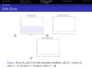
u(x, t)|x=∞ = 0, u(0, t) = b sin (ωt), t ∈ [0, T ] (30)
√ω √
− x ω bω ∞ e −ut sin x u
u(x, t) = b e 2 sin ωt − x + du
2 π 0 u2 + ω2
ω b 1
ux (0, t) = −b (sin (ωt) + cos (ωt))+ 3 +O 5 , as t → ∞
2 πωt 2 t2

26. Introduction Elliptic problem Parabolic problem Proposed Work Conclusion
Benchmarks
DtN Error
a) b)
c)
Figure: Error of ux (0, t) for the boundary condition u(0, t) = sin(t) a)
with k = 4, b) with k = 8 and c) with k = 16

27. Introduction Elliptic problem Parabolic problem Proposed Work Conclusion
Benchmarks
Benchmark 3: Diurnal Earth Heating
∂u(x, t) ∂ 2 u(x, t)
= , (x, t) ∈ [0, ∞) × [0, T ], (31)
∂t ∂x 2
u(x, 0) = 0, x ∈ [0, ∞) (32)
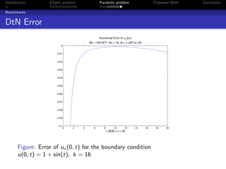
u(0, t) = 1 + b sin (ωt), t ∈ [0, T ] (33)
1 ω b
ux (0, t) ≈ − √ − b (sin (ωt) + cos (ωt)) + 3 , as t → ∞
πt 2 πωt 2

28. Introduction Elliptic problem Parabolic problem Proposed Work Conclusion
Benchmarks
DtN Error
Numerical Error of ux(0,t)
Mt = 1541877, Nx = 16, dt = 1.2971e−05
0
−0.01
−0.02
−0.03
−0.04
−0.05
−0.06
−0.07
−0.08
−0.09
−0.1
0 2 4 6 8 10 12 14 16 18 20
1.3636 < t < 20
Figure: Error of ux (0, t) for the boundary condition
u(0, t) = 1 + sin(t), k = 16

29. Introduction Elliptic problem Parabolic problem Proposed Work Conclusion
Proposed work: Crystal Growth Problem4
Infinite melt cooled below its freezing temperature. Two-phase
flow with the moving interface separating the crystal from the
melt. We wish to model the evolution of the crystal-melt interface.
Mathematical model for the problem
The diffusion equation in the melt
∂T 2
=D T, (34)
∂t
where D is constant thermal diffusivity.
The specified temperature in the melt far from the interface
T → T∞ as y → ∞ (35)
4
M. Kunka

30. Introduction Elliptic problem Parabolic problem Proposed Work Conclusion
The temperature at the interface with the parametrization
y = yi (x, t) is given by the Gibbs-Thomson relation
T = Tm (1 − γκ) on y = yi (x, t), (36)
where κ - interface curvature and γ - capillary length that
characterizes the surface tension.
And the kinematic condition relating the heat flux and the velocity
of the moving interface
∂T
cD = −Lvn on y = yi (x, t), (37)
∂n
vn - the normal velocity of the interface, L - the latent heat and c -
specific heat.

31. Introduction Elliptic problem Parabolic problem Proposed Work Conclusion
We propose to investigate the crystal growth problem in the
less well studied limit of large Peclet number. In this limit, we
expect a boundary layer adjacent to the moving interface
where the temperature gradients are large.
A singular perturbation analysis will be performed to derive a
leading order equation governing the temperature in the layer.
We propose to efficiently solve this equation with high
accuracy using optimal grids.

32. Introduction Elliptic problem Parabolic problem Proposed Work Conclusion
Conclusion
We showed that the described special choice of the
discretization grid steps provides a spectral convergence order
of the solution at the boundary.
This method of computing the Riesz transform will be applied
to a new numerical method of Ambrose and Siegel for
removing the stiffness from boundary integral calculations
with surface tension.
We propose to efficiently solve the equation for the crystal
growth problem in the limit of large Peclet number with high
accuracy using optimal grids.