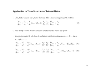
The document summarizes two models: 1. The Lo-Zivot Threshold Cointegration Model, which uses a threshold vector error correction model (TVECM) to analyze the dynamic adjustment of cointegrated time series variables to their long-run equilibrium. It allows for nonlinear and asymmetric adjustment speeds. 2. A bivariate vector error correction model (VECM) and band-threshold vector error correction model (BAND-TVECM) that extend the VECM to allow for nonlinear and discontinuous adjustments to long-run equilibrium across multiple regimes defined by thresholds on a variable. This captures asymmetric adjustment speeds and dynamic behavior. The BAND-TVECM allows modeling of

1. Model 1: Lo-Zivot Threshold Cointegration Model
• Balke and Fomby (1997):
– univariate cointegrating residual behavior
– ad hoc model selection, no specification test is provided for TAR models
• Lo and Zivot (2001):
– multivariate setting of a threshold vector error correction model (TVECM) to investigate the dynamic
adjustment of individual series more efficiently, to uncover the overall dynamics of the whole
multivariate system, capture the long-run equilibrium relationship as well as the short-term
disequilibrium adjustment process to the long-run equilibrium
– use a specification test offered by Hansen (1997, 1999) to see which TAR model is appropriate to
capture the threshold cointegration relationships for the Treasury and corporate bond rates
• A TVECM will be estimated and used to evaluate the dynamic time paths of yield
spread adjustments to U.S. Treasury and corporate bond indices which allows:
•
discontinuous adjustment relative to the thresholds
•
nonlinear adjustments to the long-run equilibrium
•
asymmetric adjusting speeds to the long-run equilibrium
1

2. A Bivariate Vector Error Correction Model (VECM)
• a bivariate vector autoregressive (VAR) model, where Xt is a 2 × 1 vector with X 't = ( x1t , x 2 t ) :
k
X t = A0 + ∑ Ai X t −i + ε t , (1)
i =1
where ε t is a 2 × 1 white noise process, k is the order of autoregressive terms, A0 is a 2 × 1 parameter vector, and
Ai’ re 2 × 2 parameter matrices
s
k −1
• ∆X t = A 0 + ΠX t −1 + ∑ Γi ∆X t − i + ε t , (2)
i =1
where Π = − ∑ A i − I 2  , and Γi = − ∑ A l , for i = 1, 2, … , k-1
k k
 
 i =1  l = i +1
• if elements of Xt are I(1) and cointegrated with a normalized cointegrating vector β ' = (1, − β 2 ) , then (2) has a vector
error-correction model (VECM) representation:
k −1
∆X t = A 0 + γβ ' X t −1 + ∑ Γi ∆X t −i + ε t , (3)
i =1
γ  γ − β 2γ 1 
where Π = γβ ' =  1 (1,− β 2 ) =  1
γ . (4)
γ 
 2  2 − β 2γ 2 

• γ is the speeds of adjustment, β ' X t −1 denotes the error-correction terms or the cointegrating residuals
2

3. The BAND-TVECM (Band-Threshold Vector Error Correction Model)
• conventional VAR and VECM can only model linear relationships
• threshold autoregression (TAR) and threshold vector error correction model (TVECM) can overcome above drawback
• TAR and TVECM have the strength of modeling nonlinear and discontinuous phenomenon
• consider a simple three-regime bivariate TVECM for the threshold cointegrating relationship of the Treasury and
corporate bond rates, express the bivariate threshold vector autoregressive (TVAR) model for Xt as:
X t = A (01) + ∑ A (i1) X t −i + ε t(1)  I 1t (z t − d ≤ c (1) )
k

 i =1


+ A (02 ) + ∑ A (i 2 ) X t − i + ε t( 2 )  I 2 t (c (1) < z t − d ≤ c ( 2 ) )
k
(5)

 i =1


A ( 3) + k A (3 ) X + ε ( 3)  I (z > c ( 2 ) ),
+
 0

∑ i t −i t  3t t − d
i =1 
where ε t( j) ’ are bivariate vector white noise processes, k is the autoregressive order, A (0j) ' s are 2 × 1 parameter
s
vectors, and A (i j) ' s are 2 × 2 parameter matrices for regime j = 1, 2, 3, and for lag i = 1, 2, … , k; zt-d is called the
threshold variable; d is called the delay parameter, d is positive and usually less than or equal to the lag length k
• in general, − ∞ = c ( 0 ) < c (1) < c ( 2 ) < c (3 ) = ∞ , the indicator function has the form:
3

4. 1, if c ( j−1) < z t − d ≤ c ( j) , j = 1, 2, 3,
I jt (c ( j −1)
< z t−d ≤c )=
( j)
(6)
0, otherwise.
• if elements of Xt are I(1) and they are cointegrated, then equation (5) can be expressed as a TVECM:
∆X t = A (01) + Π (1) X t −1 + ∑ Γi(1) ∆X t −i + ε t(1)  I 1t (z t − d ≤ c (1) )
k −1

 i =1


+ A (02) + Π ( 2) X t −1 + ∑ Γi( 2) ∆X t −i + ε t( 2)  I 2 t (c (1) < z t − d ≤ c ( 2) )
k −1
(7)

 i =1


+ A (03) + Π ( 3) X t −1 + ∑ Γi(3) ∆X t −i + ε t( 3)  I 3 t (z t − d > c ( 2) ),
k −1

 i =1


where Π ( j) = − ∑ A i( j) − I 2  , and Γi( j) = − ∑ A (l j) for regime j = 1, 2, 3, and i = 1, 2, … , k-1
k k
 
 i =1  l = i +1
• if elements of Xt are cointegrated with a common (across regime) normalized cointegrating vector β ' = (1, − β 2 ) and if
the error terms ε t( j) share the same variance-covariance structure, then the TVECM may be written as:
∆X t = A (01) + γ (1) β ' X t −1 + ∑ Γi(1) ∆X t −i  I 1t (z t − d ≤ c (1) )
k −1

 i =1


+ A (02 ) + γ ( 2) β ' X t −1 + ∑ Γi( 2 ) ∆X t − i  I 2 t (c (1) < z t − d ≤ c ( 2) )
k −1
(8)

 i =1


+ A (03) + γ ( 3) β ' X t −1 + ∑ Γi( 3) ∆X t − i  I 3 t (z t − d > c ( 2) ) + ε t ,
k −1

 i =1


4

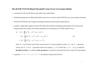
5.  γ 1( j)   γ ( j) − β 2 γ 1( j) 
where γ ( j)
β '= Π ( j)
 ( j) (1,− β 2 ) =  1( j)
= γ  , and j = 1, 2, 3 (9)
γ 2 

 2 − β 2 γ 2( j) 

• note that although the three regimes share a common cointegrating vector β ' = (1, − β 2 ) , the speeds of adjustment
γ ( j) ' = (γ 1( j) , γ 2( j) ) are regime specific. For example, we may observe that γ 1(1) ≠ γ 1( 3) or γ 2( 2 ) ≠ γ 2( 3)
• the simplest form for the TVECM occurs when k = 1 in equation (8) so that all lag difference terms drop out of the
equation, the cointegrating residual β ' X t follows a regime specific AR(1) process or threshold autoregressive (TAR)
process:
β ' X t = δ ( j) + ρ ( j) β ' X t −1 + η t( j) ,
with ρ ( j) = 1 + β ' γ ( j) = 1 + γ 1( j) − β 2 γ 2( j) , where δ ( j) = β ' A (0j) and η t( j) = β ' ε t( j)
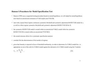
Proof:
Set k = 1 in equation (8) to obtain:
∆X t = X t − X t −1 = [A (01) + γ (1)
β ' X t −1 ]I 1t (z t − d ≤ c (1) ) + [A (02 ) + γ ( 2) β ' X t −1 ]I 2 t (c (1) < z t − d ≤ c ( 2 ) )
+ [A (03) + γ ( 3 ) β ' X t −1 ]I 3 t (z t − d > c ( 2 ) ) + ε t .
Multiply both sides by β ' , then move β ' Xt-1 to the right-hand side, will obtain:
β ' X t = β ' X t −1 + [β ' A (01) + β ' γ (1) β ' X t −1 ]I 1t ( z t −d ≤ c (1) ) + [β ' A (02 ) + β ' γ ( 2 ) β ' X t −1 ]I 2 t (c (1) < z t −d ≤ c ( 2 ) )
+ [β ' A (03 ) + β ' γ (3 ) β ' X t −1 ]I 3 t ( z t −d > c ( 2 ) ) + β ' ε t .
5

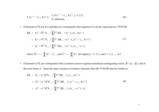
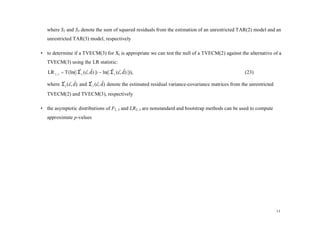
6. Split β ' X t −1 and ε t to each regime, then obtain:
β ' X t = [β ' A (01) + β ' X t −1 + β ' γ (1) β ' X t −1 + β ' ε t(1) ]I1t (z t − d ≤ c(1) )
+ [β ' A (02 ) + β ' X t −1 + β ' γ ( 2 ) β ' X t −1 + β ' ε t( 2 ) ]I 2 t (c(1) < z t − d ≤ c ( 2 ) )
+ [β ' A (03 ) + β ' X t −1 + β ' γ ( 3) β ' X t −1 + β ' ε t(3 ) ]I3 t ( z t − d > c ( 2 ) ).
Collect terms to get:
β ' X t = [β ' A (01) + (1 + β ' γ (1) ) β ' X t −1 + β ' ε t(1) ]I1t ( z t − d ≤ c (1) )
+ [β ' A (02 ) + (1 + β ' γ ( 2 ) ) β ' X t −1 + β ' ε t( 2 ) ]I 2 t (c (1) < z t − d ≤ c( 2 ) )
+ [β ' A (03 ) + (1 + β ' γ ( 3) ) β ' X t −1 + β ' ε t( 3) ]I3 t (z t − d > c( 2 ) )
= δ ( j) + ρ ( j ) β ' X t −1 + η t( j ) .
Q.E.D.
• β ' X t is stable within each regime if the stability condition ρ ( j) = 1 + γ 1( j) − β 2 γ 2( j) < 1 holds for each regime
• in equation (8), with k = 1, then we have:
∆X t = [A (01) + γ (1) β ' X t −1 ]I 1t (z t − d ≤ c (1) ) + [A (02 ) + γ ( 2)
β ' X t −1 ]I 2 t (c (1) < z t − d ≤ c ( 2) )
(10)
+ [A (03 ) + γ ( 3 ) β ' X t −1 ]I 3 t (z t − d > c ( 2 ) ) + ε t .
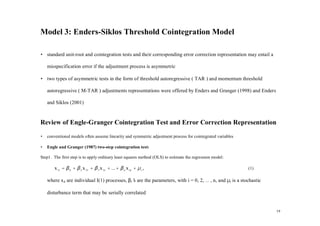
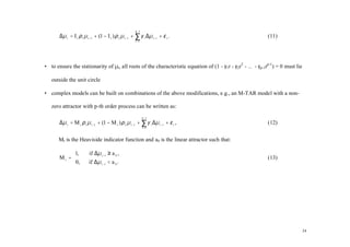
• it is easier to capture the long-run equilibrium relationship if we rewrite (10) in:
∆X t = γ (1) [β ' X t −1 − µ (1) ]I 1t ( z t − d ≤ c (1) ) + γ ( 2 ) [β ' X t −1 − µ ( 2) ]I 2 t (c (1) < z t − d ≤ c ( 2 ) )
(11)
+ γ ( 3) [β ' X t −1 − µ ( 3) ]I 3t (z t − d > c ( 2) ) + ε t .
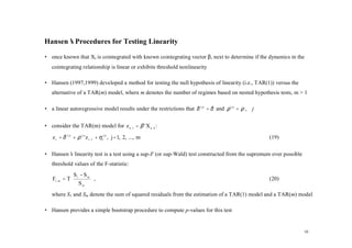
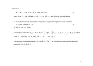
explicitly we have:
6

7. γ 1(1) [x 1t −1 − β 2 x 2 t −1 − µ (1) ] + ε 1(t1) , if z t − d ≤ c (1) ,

∆x 1t = γ 1( 2 ) [x 1t −1 − β 2 x 2 t −1 − µ ( 2 ) ] + ε 1(t2 ) , if c (1) < z t − d ≤ c ( 2 ) , and
γ ( 3 ) [x − β x − µ ( 3) ] + ε 1(t3 ) , if z t − d > c ( 2 ) ,
 1 1t −1 2 2 t −1
γ 2(1) [x 1t −1 − β 2 x 2 t −1 − µ (1) ] + ε 2(1t ) , if z t − d ≤ c (1) ,

∆x 2 t = γ 2( 2 ) [x 1t −1 − β 2 x 2 t −1 − µ ( 2 ) ] + ε 2( 2 ) ,
t
if c (1) < z t − d ≤ c ( 2 ) ,
γ ( 3 ) [x − β x − µ ]+ ε 2 t ,
( 3) (3)
if z t − d > c ( 2 ) .
 2 1t −1 2 2 t −1
• the magnitudes and signs of the γ’ will provide fruitful information regarding the equilibrium relationships
s
• equation (11) offers the regime-specific means µ ( j) , which is calculated as:
β ' A (0j) A (0j,1 − β 2 A (0j,)2
)
δ ( j)
µ ( j)
=− = − ( j) = , (12)
β ' γ ( j) γ 1 − β 2 γ 2( j) 1 − ρ ( j)
where A (0j) ' = (A (0j,1 , A (0j,)2 ) , and β ' = (1, − β 2 )
)
• it is also possible to eliminate the regime specific drift in Xt through the restriction:
A (0j) = −γ ( j) µ ( j) (13)
where µ ( j) is calculated by (12)
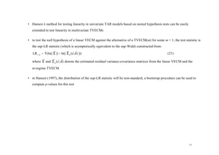
• note that we may rewrite equation (11) as follows with z t −1 = β ' X t −1 = x 1t −1 − β 2 x 2 t −1 :
7

8. γ (1)
[z t −1
− µ (1 ) ] + ε t , if z t −d ≤ c (1) ,

∆X t = γ (2)
[z t −1 − µ (2) ] + ε t , if c (1) < z t − d ≤ c ( 2 ) , (14)
γ

( 3)
[z t −1
− µ ( 3) ] + ε t , if z t − d > c ( 2 ) .
• consider the case of d = 1, γ ( 2 ) = 0 and A (02 ) = 0 in equation (14), this is the Band-TVECM structure which is the most
popular form in threshold cointegrating applications:
γ (1) [z t −1 − µ (1) ] + ε t , if z t −1 ≤ c (1) ,

∆X t = ε t , if c (1) < z t −1 ≤ c ( 2 ) , (15)
γ ( 3 ) [z − µ ( 3 ) ] + ε , if z t −1 > c ( 2 ) .
 t −1 t
• the stability conditions must hold for the outer regimes, i.e., ρ ( j) = 1 + γ 1( j) − β 2 γ 2( j) < 1, for j = 1 and 3
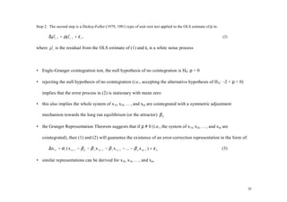
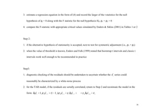
• one may interpret above model as:
1. if the cointegrating residual (the error-correction term) z t −1 = β ' X t −1 lies within the inner band [c (1) , c ( 2 ) ] , then Xt
behaves like a random walk process without the drift, i.e., ∆X t has no tendency reverting to any long-term
equilibrium
2. if z t −1 is less than c (1) , then z t reverts to the regime specific mean µ (1) with adjustment coefficient ρ (1) while ∆X t
adjusts with speed of adjustment vector γ (1)
8

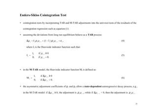
9. 3. if z t −1 is greater than c ( 2 ) , then z t reverts to the regime specific mean µ ( 3) with adjustment coefficient ρ ( 3) and
∆X t adjusts with speed of adjustment vector γ ( 3 )
4. expect γ i( 3) ≤ 0, γ i(1) > 0, for i = 1, 2, because of the force of the error correcting toward the long-term equilibrium
• if the regime specific means of the cointegrating residual z t are equal to the nearby threshold values (it is called the
“continuous”model): µ (1) = c (1) , µ ( 3) = c ( 2 ) , then (15) may be written as:
γ (1) [z t −1 − c (1) ] + ε t , if z t −1 ≤ c (1) ,

∆X t = ε t , if c (1) < z t −1 ≤ c ( 2 ) , (16)
γ ( 3) [z − c ( 2 ) ] + ε , if z t −1 > c ( 2 ) .
 t −1 t
• the “symmetric”threshold model arises when the threshold values are symmetric against the origin ( c ( 2 ) = −c(1) = c ):
γ (1) [z t −1 + c] + ε t , if z t −1 ≤ −c,

∆X t = ε t , if − c < z t −1 ≤ c, (17)
γ ( 3) [z − c] + ε , if z t −1 > c .
 t −1 t
• if µ (1) = µ (3 ) = 0, then we have the EQ-TVECM:
γ (1) z t −1 + ε t , if z t −1 ≤ c (1) ,

∆X t = ε t , if c (1) < z t −1 ≤ c ( 2 ) , (18)
γ ( 3 ) z + ε , if z t −1 > c ( 2 ) .
 t −1 t
9

10. Hansen’ Procedures for Testing Linearity
s
• once known that Xt is cointegrated with known cointegrating vector β, next to determine if the dynamics in the
cointegrating relationship is linear or exhibits threshold nonlinearity
• Hansen (1997,1999) developed a method for testing the null hypothesis of linearity (i.e., TAR(1)) versus the
alternative of a TAR(m) model, where m denotes the number of regimes based on nested hypothesis tests, m > 1
• a linear autoregressive model results under the restrictions that δ ( j) = δ and ρ ( j) = ρ , ∀j
• consider the TAR(m) model for z t −1 = β ' X t −1 :
z t = δ ( j) + ρ ( j) z t −1 + η t( j) , j = 1, 2, ..., m (19)
• Hansen’ linearity test is a test using a sup-F (or sup-Wald) test constructed from the supremum over possible
s
threshold values of the F-statistic:
 S − Sm 
F1, m = T 1
 S ,
 (20)
 m 
where S1 and Sm denote the sum of squared residuals from the estimation of a TAR(1) model and a TAR(m) model
• Hansen provides a simple bootstrap procedure to compute p-values for this test
10

11. • Hansen’ method for testing linearity in univariate TAR models based on nested hypothesis tests can be easily
s
extended to test linearity in multivariate TVECMs
• to test the null hypothesis of a linear VECM against the alternative of a TVECM(m) for some m > 1, the test statistic is
the sup-LR statistic (which is asymptotically equivalent to the sup-Wald) constructed from:
LR 1, m = T(ln(| Σ |) − ln(| Σ m (c, d ) |))
ˆ ˆ ˆˆ (21)
where Σ and Σ m (c, d) denote the estimated residual variance-covariance matrices from the linear VECM and the
ˆ ˆ ˆˆ
m-regime TVECM
• in Hansen (1997), the distribution of the sup-LR statistic will be non-standard, a bootstrap procedure can be used to
compute p-values for this test
11

12. Hansen’ Procedures for Model Specification Test
s
• Hansen (1999) uses a sequential testing procedure based on nested hypotheses, we will adopt his nested hypotheses
tests based on unrestricted estimation of TAR models and TVECMs
• start with a typical three-regime continuous symmetric threshold and symmetric adjustment BAND-TAR model for zt
as well as a three-regime symmetric threshold and symmetric adjustment BAND-TVECM for Xt
• the symmetric BAND-TAR model is nested within an unrestricted TAR(3) model while the symmetric
BAND-TVECM is nested within an unrestricted TVECM(3)
• this nested structure allows for a systematic specification analysis
• consider first the determination of the number of regimes
• given that linearity is rejected in favor of threshold nonlinearity, in order to determine if a TAR(3) model for zt is
appropriate we test of the null of a TAR(2) model against the alternative of a TAR(3) model using the F-statistic:
 S − S3 
F2 , 3 = T 2
 S ,  (22)
 3 
12

13. where S2 and S3 denote the sum of squared residuals from the estimation of an unrestricted TAR(2) model and an
unrestricted TAR(3) model, respectively
• to determine if a TVECM(3) for Xt is appropriate we can test the null of a TVECM(2) against the alternative of a
TVECM(3) using the LR statistic:
LR 2 , 3 = T (ln(| Σ 2 (c, d) |) − ln(| Σ 3 (c, d) |)),
ˆ ˆˆ ˆ ˆˆ (23)
where Σ 2 (c, d ) and Σ 3 (c, d ) denote the estimated residual variance-covariance matrices from the unrestricted
ˆ ˆˆ ˆ ˆˆ
TVECM(2) and TVECM(3), respectively
• the asymptotic distributions of F2, 3 and LR2, 3 are nonstandard and bootstrap methods can be used to compute
approximate p-values
13

14. Model 2: Hansen-Seo Two-Regime Threshold Cointegartion Model
• Hansen and Seo (2001) propose a formal test procedure for threshold cointegration and they offer an algorithm to estimate model
parameters
• A two-regime vector error correction model with one cointegrating vector and with one built-in threshold effect in the error-
correction term
• Based on a fully specified joint model, they derive the maximum likelihood estimator of a threshold cointegration model
• Under the null hypothesis of linearity the threshold parameter is not identified, which causes a nuisance parameter problem, they
then:
1. base inference on a Sup-LM (Lagrange Multiplier) test statistic
2. derive the asymptotic null distribution for test statistic and discuss bootstrap approximations to the
sampling distribution: (a) the fixed regressor bootstrap
(b) the residual-based bootstrap
14

15. Two-Regime Threshold Cointegration Model
• xt is a p × 1 I(1) with one p × 1 cointegrating vector β, w t ( β ) = β ' x t denotes the I(0) error-correction term
• A linear vector error correction model (VECM) of order (L+1):
∆x t = A ' X t −1 ( β ) + u t , (1)
where X 't −1 ( β ) = [ 1, w t −1 ( β ), ∆x t −1 , ∆x t − 2 , ..., ∆x t − L ], with dimensions: Xt-1(β) is k × 1, k = p × L + 2, A is k ×
p
• The error term ut is a p × 1 Martingale difference sequence with finite variance-covariance matrix Σ = E(u t u 't ) of
dimension p × p
• The approach is to estimate the parameters (β, A, Σ) by maximum likelihood estimation given the assumption
that the error terms u t’ are i.i.d. Gaussian distributed
s
• Let γ be the threshold parameter, a two-regime threshold cointegration model:
A 1' X t −1 ( β ) + u t , if w t −1 ( β ) ≤ γ ,
∆x t =  ' ,
A 2 X t −1 ( β ) + u t , if w t −1 ( β ) > γ ,
15

16. or rewrite as
∆x t = A 1' X t −1 ( β )d 1t ( β , γ ) + A '2 X t −1 ( β )d 2 t ( β , γ ) + u t , (2)
where d 1 t ( β , γ ) = I( w t −1 ( β ) ≤ γ ) , d 2 t ( β , γ ) = I( w t −1 ( β ) > γ ) , and I(⋅) is the indicator function
• To ensure the nonlinearity, Hansen-Seo among others suggest imposing the boundary constraint:
π 0 ≤ Pr( w t −1 ( β ) ≤ γ ) ≤ 1 − π 0 (3)
we will set 0.05 ≤ π 0 ≤ 0.15
n 1 n
• The likelihood function is: L n (A 1 , A 2 , Σ, β , γ ) = − log Σ − ∑ u t (A 1 , A 2 , β , γ )' Σ −1 u t ( A 1 , A 2 , β , γ ), where:
2 2 t =1
u t ( A 1 , A 2 , β , γ ) = ∆x t − A 1 X t −1 ( β )d 1 t ( β , γ ) − A '2 X t −1 ( β )d 2 t ( β , γ )
'
• The maximum likelihood estimators (MLEs) ( A 1 , A 2 , Σ, β , γˆ are the values that maximize the likelihood
ˆ ˆ ˆˆ )
function L n (A 1 , A 2 , Σ, β , γ )
16

17. Estimation Procedure:
• First concentrate out ( A 1 , A 2 , Σ) by holding ( β , γ ) fixed and compute the constrained MLE for ( A1 , A 2 , Σ)
• Through OLS estimation, since given Gaussian error terms the maximum likelihood estimators are the
same as ordinary least squared estimators:
−1
A 1 ( β , γ ) =  ∑ X t −1 ( β ) X t −1 ( β ) ' d 1t ( β , γ )   ∑ X t −1 ( β ) ∆x t d 1t ( β , γ )  ,
n n
ˆ     (4)
 t =1   t =1 
−1
A 2 ( β , γ ) =  ∑ X t −1 ( β )X t −1 ( β ) ' d 2 t ( β , γ )   ∑ X t −1 ( β )∆x t d 2 t ( β , γ )  ,
n n
ˆ     (5)
 t =1   t =1 
1 n
u t ( β , γ ) = u t (A 1 ( β , γ ), A 2 ( β , γ ), β , γ ) , and Σ( β , γ ) = ∑ u t ( β , γ )u t ( β , γ ) ' .
ˆ ˆ ˆ ˆ ˆ ˆ (6)
n t =1
• The concentrated likelihood function is:
n np
L n ( β , γ ) = L n ( A 1 ( β , γ ), A 2 ( β , γ ), Σ( β , γ ), β , γ ) = − log Σ( β , γ ) − .
ˆ ˆ ˆ ˆ (7)
2 2
• Compute the vector of parameters: ( β , γˆ .
ˆ )
• The MLE u t = u t ( β , γˆ are the minimizers of log Σ( β , γ ) subject to the boundary constraint (3).
ˆ ˆ ˆ ) ˆ
• The MLE for A1 and A2 are then: A 1 = A 1 ( β , γˆ and A 2 = A 2 ( β , γˆ .
ˆ ˆ ˆ ) ˆ ˆ ˆ )
17

18. Application to Term Structure of Interest Rates:
• Let x1t be the long rate and x2t be the short rate. Then a linear cointegrating VAR model is:
 ∆x 1 t   µ 1   α 1  Γ Γ12  ∆x 1t −1   u 1t 
  =   +  ( x 1t −1 − βx 2 t −1 ) +  11
 ∆x   µ   α  Γ  +  (8)
 2t   2   2   21 Γ22  ∆x 2 t −1   u 2 t 
   
• Note: if set β = 1, then the error-correction term becomes the interest rate spread
• A two-regime model H1 will allow all coefficients to differ depending upon x 1t −1 − βx 2 t −1 ≤ γ or
x 1t −1 − βx 2 t −1 > γ :
 ∆x 1 t   µ 1   α 1   Γ (1) Γ121)  ∆x 1t −1   u 1t 
(1) (1 ) (
  (1)  +  (1) ( x 1t −1 − βx 2 t −1 ) +  111)
 ∆x  =  µ   α 
   +   , if x 1t −1 − βx 2 t −1 ≤ γ , (9a)
 2t   2   2 
Γ(
 21 Γ22 )  ∆x 2 t −1   u 2 t 
(1
   
 ∆x 1t   µ 1  α 1   Γ ( 2) Γ122 )  ∆x 1t −1   u 1t 
(2) (2) (
  =  ( 2 )  +  ( 2 ) ( x 1t −1 − βx 2 t −1 ) +  112 )
 ∆x   µ  α    +   , if x 1t −1 − βx 2 t −1 > γ (9b)
 2t   2   2 
Γ(
 21 Γ222 )  ∆x 2 t −1   u 2 t 
(
   
18

19. Model 3: Enders-Siklos Threshold Cointegration Model
• standard unit-root and cointegration tests and their corresponding error correction representation may entail a
misspecification error if the adjustment process is asymmetric
• two types of asymmetric tests in the form of threshold autoregressive ( TAR ) and momentum threshold
autoregressive ( M-TAR ) adjustments representations were offered by Enders and Granger (1998) and Enders
and Siklos (2001)
Review of Engle-Granger Cointegration Test and Error Correction Representation
• conventional models often assume linearity and symmetric adjustment process for cointegrated variables
• Engle and Granger (1987) two-step cointegration test:
Step1. The first step is to apply ordinary least squares method (OLS) to estimate the regression model:
x 1t = β 0 + β 2 x 2 t + β 3 x 3 t + ... + β n x nt + µ t , (1)
where xit are individual I(1) processes, βi’ are the parameters, with i = 0, 2, … , n, and µt is a stochastic
s
disturbance term that may be serially correlated
19

20. Step 2. The second step is a Dickey-Fuller (1979, 1981) type of unit root test applied to the OLS estimate of ρ in:
∆µ t −1 = ρµ t −1 + ε t ,
ˆ ˆ (2)
where µ t is the residual from the OLS estimate of (1) and εt is a white noise process
ˆ
• Engle-Granger cointegration test, the null hypothesis of no cointegration is H0: ρ = 0
• rejecting the null hypothesis of no cointegration (i.e., accepting the alternative hypothesis of HA: – < ρ < 0)
2
implies that the error process in (2) is stationary with mean zero
• this also implies the whole system of x 1t, x2t, … , and xnt are cointegrated with a symmetric adjustment
mechanism towards the long run equilibrium (or the attractor) β 0
• the Granger Representation Theorem suggests that if ρ ≠ 0 (i.e., the system of x1t, x2t, … , and xnt are
cointegrated), then (1) and (2) will guarantee the existence of an error-correction representation in the form of:
∆x 1t = α 1 ( x 1 t −1 − β 0 − β 2 x 2 t −1 − β 3 x 3 t −1 − ... − β n x nt −1 ) + ε 1t (3)
• similar representations can be derived for x2t, x3t, … , and xnt
20

21. Enders-Siklos Cointegration Test
• cointegration tests by incorporating TAR and M-TAR adjustments into the unit-root tests of the residuals of the
cointegration regression such as equation (1)
• assuming the deviations from long run equilibrium behave as a TAR process:
∆µ t = I t ρ 1 µ t −1 + (1 − I t ) ρ 2 µ t −1 + ε t , (4)
where It is the Heaviside indicator function such that:
1, if µ t −1 ≥ 0
It =  (5)
0, if µ t −1 < 0.
• in the M-TAR model, the Heaviside indicator function Mt is defined as:
1, if ∆µ t −1 ≥ 0
Mt =  (6)
0, if ∆µ t −1 < 0.
• the asymmetric adjustment coefficients of ρ1 and ρ2 allow a state-dependent autoregressive decay process, e.g.,
in the M-TAR model: if ∆µ t −1 ≥ 0 , the adjustment is ρ 1 µ t −1 ; while if ∆µ t − 1 < 0, then the adjustment is ρ 2 µ t −1
21

22. Example: consider the TAR model, equations (4) and (5): the autoregressive decay to depend on µt-1
1. if |ρ2| > |ρ1|, say ρ1 = -0.2, ρ2 = -0.8, then positive deviations from the long-run cointegration equilibrium are
more persisted than negative deviations
2. there is a slow adjustment when the equilibrium error is above the attractor, while there is an accelerated
adjustment when the equilibrium error is below the attractor
3. this adjustment mechanism captures the feature of “deep”cyclical processes documented by Sichel (1993)
Example: consider the M-TAR model, equations (4) and (6): the autoregressive decay to depend on ∆µt-1
1. if |ρ2| > |ρ1|, say, ρ1 = -0.2, ρ2 = -0.8, there is little decay when ∆µt-1 is positive but substantial decay when ∆µt-1
is negative; then increases tend to persist but decreases tend to revert quickly toward the attractor
2. the M-TAR model could easily capture the “sharp”movements documented in DeLong and Summer (1986) and
Sichel (1993)
22

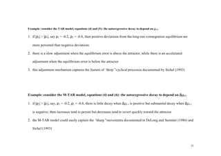
23. Extensions to modify the basic threshold cointegration model:
(1) allow a non-zero drift term as the linear attractor, which can be expressed as:
∆µ t = I t ρ 1 ( µ t −1 − a 0 ) + (1 − I t ) ρ 2 ( µ t −1 − a 0 ) + ε t , (7)
where It is the Heaviside indicator function such that:
1, if µ t −1 ≥ a 0
It =  (8)
0, if µ t −1 < a 0 .
(2) allow a drift and linear trend as attractor with the expression:
∆µ t = I t ρ 1 [ µ t −1 − a 0 − a 1 ( t − 1)] + (1 − I t ) ρ 2 [ µ t −1 − a 0 − a 1 ( t − 1)] + ε t , (9)
where It is the Heaviside indicator function such that:
1, if µ t −1 ≥ a 0 + a 1 ( t − 1)
It =  (10)
0, if µ t −1 < a 0 + a 1 ( t − 1).
(3) involve higher-order terms of the error process to purge possible auto-correlation:
23

24. p −1
∆µ t = I t ρ 1 µ t −1 + (1 − I t ) ρ 2 µ t −1 + ∑ γ i ∆µ t − i + ε t . (11)
i =1
• to ensure the stationarity of µt, all roots of the characteristic equation of (1 - γ1r - γ2r2 - … - γp-1rp-1) = 0 must lie
outside the unit circle
• complex models can be built on combinations of the above modifications, e.g., an M-TAR model with a non-
zero attractor with p-th order process can be written as:
p −1
∆µ t = M t ρ 1 µ t −1 + (1 − M t ) ρ 2 µ t −1 + ∑ γ i ∆µ t −i + ε t , (12)
i =1
Mt is the Heaviside indicator function and a0 is the linear attractor such that:
1, if ∆µ t −1 ≥ a 0 ,
Mt =  (13)
0, if ∆µ t −1 < a 0 .
24

25. Chan’ consistent estimator of the threshold
s
• Tsay (1989) and Chan (1993) offer methodologies if the underlying variables are within the threshold
autoregressive framework
• Tong (1983) also demonstrates that if the adjustment process is asymmetric then the sample mean is a biased
estimator of the attractor
• Chan (1993) shows that searching over all values of a0 so as to minimize the sum of squared errors from the
fitted model yields a super-consistent estimator of the threshold
Estimation Procedures
Case 1: τ equals 0
Step1:
1. regress one of the variables on a constant and the other variable(s) and save the residuals sequence { µ t }
ˆ
2. set the Heaviside indicator function according to (5) or (6) using τ = 0
25

26. 3. estimate a regression equation in the form of (4) and record the larger of the t statistics for the null
hypothesis of ρi = 0 along with the F statistic for the null hypothesis H0: ρ1 = ρ2 = 0
4. compare the F-statistic with appropriate critical values simulated by Enders & Siklos (2001) in Tables 1 or 2
Step 2:
1. if the alternative hypothesis of stationarity is accepted, next to test for symmetric adjustment (i.e., ρ1 = ρ2)
2. when the value of threshold is known, Enders and Falk (1999) stated that bootstrap t intervals and classic t
intervals work well enough to be recommended in practice
Step3:
1. diagnostic checking of the residuals should be undertaken to ascertain whether the ε t series could
ˆ
reasonably be characterized by a white-noise process
2. for the TAR model, if the residuals are serially correlated, return to Step 2 and reestimate the model in the
form: ∆µ t = I t ρ 1 µ t −1 + (1 − I t ) ρ 2 µ t −1 + γ 1 ∆µ t −1 + ⋅ ⋅ ⋅ + γ p ∆µ t − p + ε t
ˆ ˆ ˆ ˆ ˆ
26

27. 3. for the M-TAR case, replace It with Mt as specified in (6)
4. lag lengths can be determined by an analysis of the regression residuals and using model-selection criteria
such as AIC/BIC
27

28. Case 2: τ is unknown
Step 1:
regress one of the variables on a constant and the other variable(s) and save the residuals sequence { µ t }
ˆ
Step 2:
1. for TAR case, the estimated residual series is sorted in ascending order and called µ 1τ < µ 2 < ⋅ ⋅ ⋅ < µ T , where
τ τ
T denotes the number of usable observations
2. discard the largest and smallest 15% of the {µ iτ } values and each of the remaining 70% of the values were
considered as possible thresholds
Step 3:
1. for each of these possible thresholds, estimate an equation in the form of (4) and (5)
28

29. 2. the estimated threshold yielding the lowest residual sum of squares is the appropriate estimate of the
threshold
3. for the M-TAR case, the potential thresholds are ∆µ 1τ , ∆µ 2 , ⋅ ⋅⋅, ∆µ T such that ∆µ 1τ < ∆µ 2 < ⋅ ⋅ ⋅ < ∆µ T
τ τ τ τ
4. for each of these possible thresholds, estimate an equation in the form of (4) and (6)
5. the estimate of the threshold is the estimated threshold yielding the lowest residual sum of squares
Step 4:
reestimate the model by incorporating the estimated threshold
Step 5:
1. inference concerning the individual values of ρ 1 and ρ 2 , and the restriction ρ 1 = ρ 2 , is problematic when
the true value of the threshold τ is unknown
29

30. 2. since the property of asymptotic multivariate normality has not been established for this case, Chan and
Tong (1989) conjectured that utilizing a constant estimate should establish the asymptotic normality of the
coefficients
3. Enders and Falk (1999) found that the inversion of the bootstrap distribution for the likelihood ratio statistic
provides reasonably good coverage in small samples
Next, to perform the following tests:
1. Estimate error-correction model by incorporating the asymmetric adjustment
2. Estimate error-correction model based on Engle-Granger symmetric adjustment method
3. Conduct forecasting performance evaluation and simulation of Enders-Siklos method versus Engle-
Granger method
30