Downloaded 15 times


![Generation of Line using Bresenham’s Principle
(Derivation, Algorithm, Flow Chart, C-Programme and its
Output)
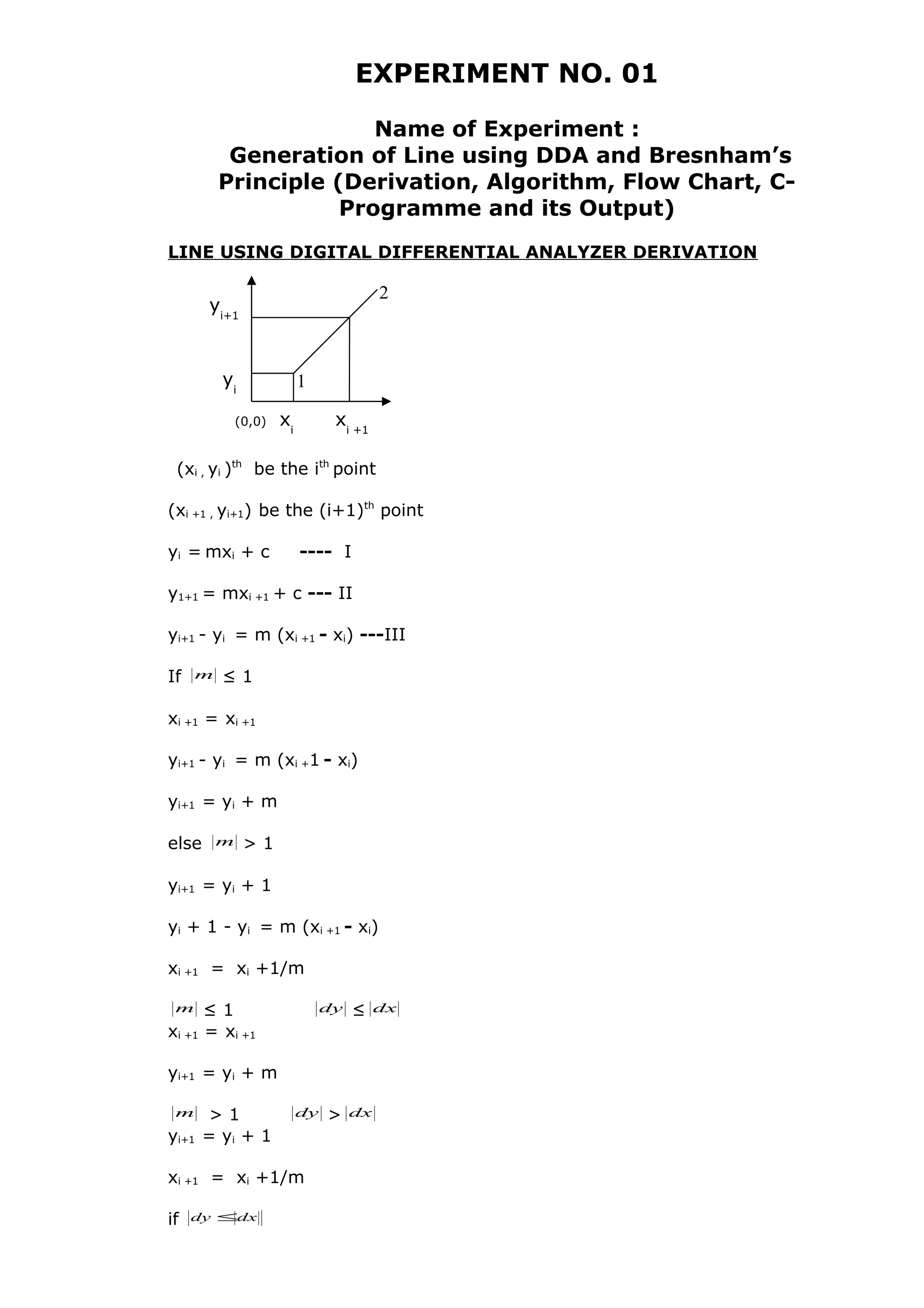
LINE USING BRESENHAM’S PRINCIPLE DERIVATION:
Let (Xi,Yi) be ith
pixel closed to the line & (Xi+1, Yi+1) be (i+1)th
pixel closed to
the line.
As m < 1
Xi+1 = Xi + 1
Yi+1 = Yi OR Yi +1
If (d1) ≤ (d2)
Yi+1 = Yi +1
If (d1 - d2) ≤0
Yi+1 = Yi
Else (d1 - d2) >0
Yi+1 = Yi +1
d1= Y- Yi
d2 = (Yi +1)-Y
(d1 - d2) = Y- Yi – (Yi+1) +Y
Yi+1 = Yi +1
= Y- Yi – Yi -1-Y
= 2Y-2Yi -1
Y=mx + c
X = Xi + 1
(d1 - d2) =2[m(Xi + 1) + c)]-2Yi -1
(d1 - d2) =2mXi+2m + 2c -2Yi -1
(d1 - d2) =2Yi Xi - 2Yi + (2Yi +2c-1)
(d1 - d2)= 2mXi - 2Yi +k
Where k = 2m + 2c-1
But m = dy/dx
(d1 - d2) =2(
dx
dy
)Xi - 2Yi +k
dx(d1 - d2) = 2dyXi - 2Yidx + kdx
Since dx is positive sign of (d1 - d2)will be the same as sign of dx (d1 - d2)
Hence dx(d1 - d2) can be taken as a decision parameter is to decide co-
ordinate of Yi +1
dx(d1 - d2) = Pi
Pi = 2dyXi - 2Yidx + k--------I
If Pi ≤0
Xi+1 = Xi + 1
Yi+1 = Yi
If Pi >0
Xi+1 = Xi + 1
Yi+1 = Yi +1
Similarly decision variable based (i+1)th
point
Pi+1= 2dyXi+1 -2Yi+1dx +k-----II
(0,0) xi
xi +1
yi+1
yi
1
2
d1
d2
Xm, Ym](https://image.slidesharecdn.com/camdpractical-150318103014-conversion-gate01/75/Computer-Aided-Manufacturing-Design-10-2048.jpg)
![As m<1
xi+1 = xi + 1
Yi+1 = Yi or Yi+1
If (d1) > (d2)
Yi+1 = Yi
If (d1) < (d2)
Yi+1 = Yi + 1
{ If (d1-d2}<0
Yi+1 = Yi
If (d1-d2}>0
Yi+1 = Yi + 1}
d1 = Y - Yi
d2 = Yi + 1 - Y
(d1 – d2) = Y - Yi – ( Yi + 1) + Y
=2Y – 2Yi – 1
Y= mX + C
X= Xi + 1
(d1 – d2) = 2[m(Xi + 1) + C ] – 2Yi 1
=2mXi – 2Yi + 2m + 2C + 1
(d1 – d2) = 2mXi – 2Yi + K
m = dy/dx
dX (d1 – d2) = 2dY Xi – 2 Yi dX + K dX
since dX be the d1 – d2 will be the same as sign of dX (d1 – d2).
Hence dX (d1 – d2) can be taken as a decision parameter co-ordiante of (Yi +
1)
dX (d1 – d2) = Pi
Pi = 2 dY Xi – 2 Yi dX + K
{If Pi < 0
xi+1 = Xi + 1
Yi+1 = Yi
If Pi > 0
Xi+1 = Xi + 1
Yi+1 = Yi + 1}
Similarly decision variables base on (i+1)th
point
Pi+1 = 2 dY Xi+1 – 2 dX Yi+1 + K
(Pi+1 – P1) = 2 dY (Xi+1 –Xi) – 2 dX (Yi+1 – Yi)
Pi+1 = Pi + 2 dY (Xi+1 –Xi) – 2 dX (Yi+1 – Yi)_____________1
If Pi < 0
xi+1 = Xi + 1
Yi+1 = Yi
Pi = Pi + 2 dY (Xi +1 –Xi) – 2 dX (Yi – Yi)
Pi = Pi +2dY
If Pi>0
xi+1 = Xi + 1
Yi+1 = Yi + 1
Pi = Pi + 2 dY (Xi +1 –Xi) – 2 dX (Yi + 1 – Yi)
Pi = Pi +2dY – 2dX
For Ist
point,](https://image.slidesharecdn.com/camdpractical-150318103014-conversion-gate01/75/Computer-Aided-Manufacturing-Design-16-2048.jpg)


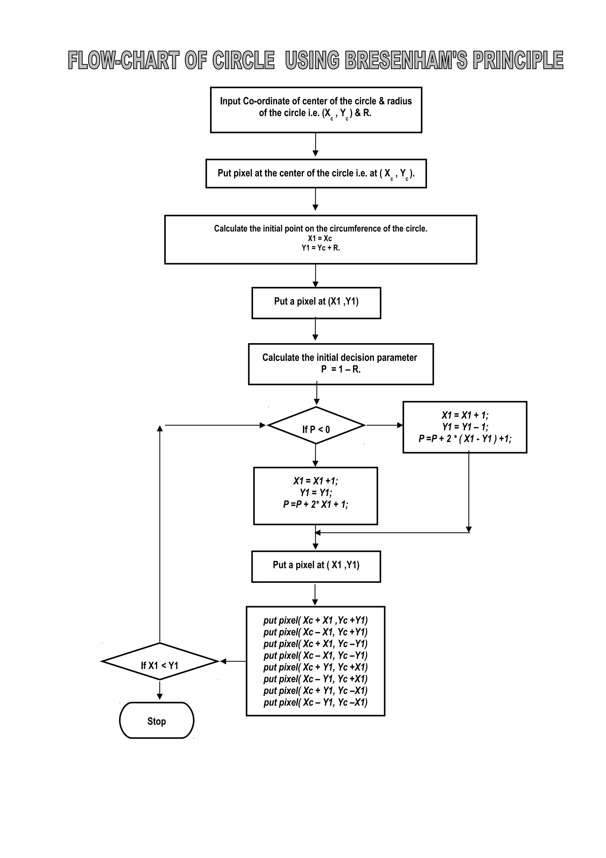
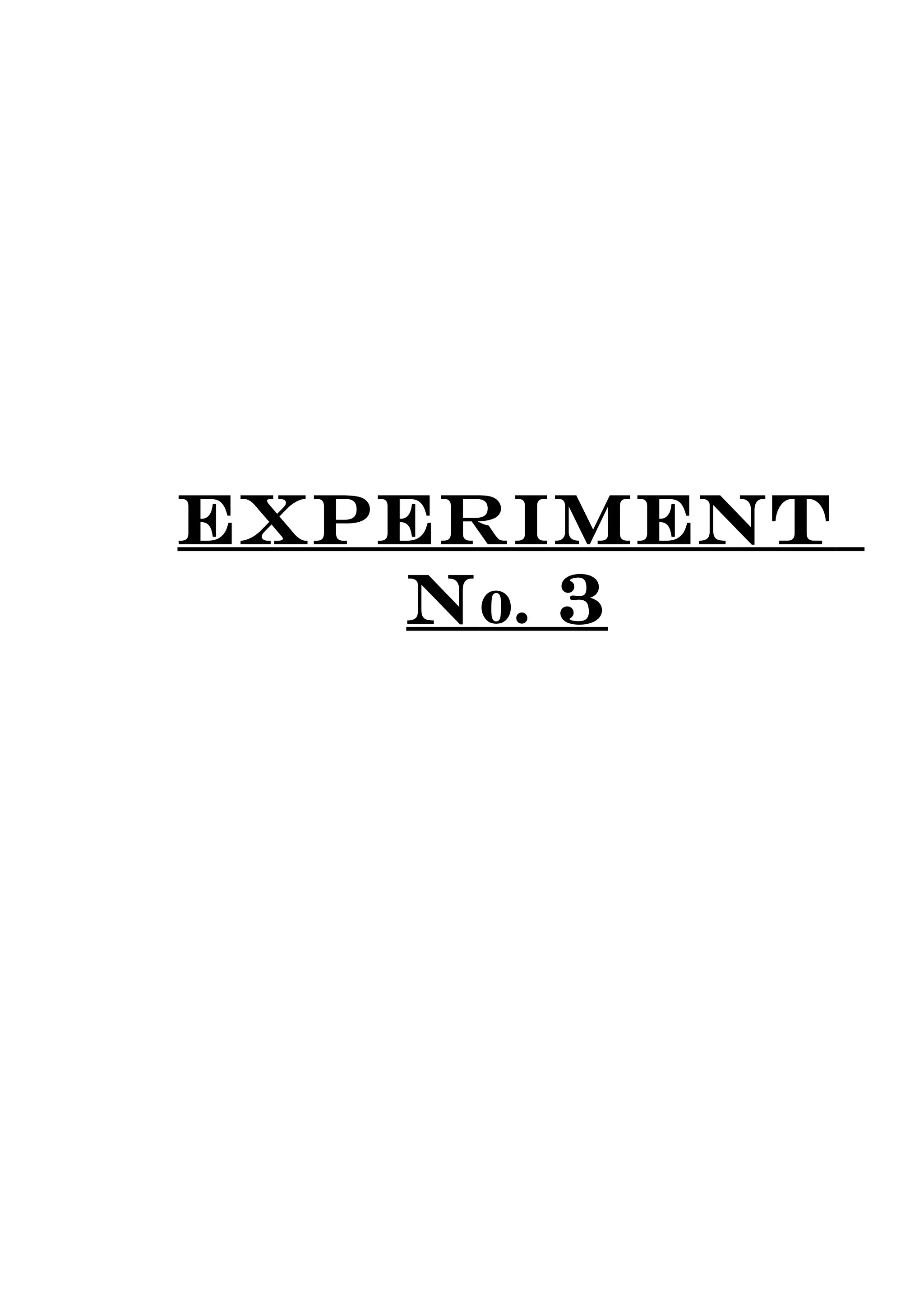
![Name of Experiment : Generation of Circle using
Parametric Bresenham’s Principle (Derivation,
Algorithm, Flow Chart, C-Programme and its Output)
CIRCLE USING BRESENHAM’S PRINCIPLE
DERIVATION: Mid point Algorithm for Generation of Circle Using
Bresenham’s Principle.
As m <1
Xi+1 = Xi +1
Yi+1 = Yi or Yi -1
Mid point m (Xm,Ym) = (Xi+1 ,Yi – ½)
If mid point inside the circle
Yi+1 = Yi
Out side the circle
Yi+1 = Yi - 1
Equation of circle = X2
+Y2
= R2
X2
+ Y2
– R2
= 0------I
Substitute the Co-ordinates of the mid point in Equation –1
Pi = Xm
2
+ Ym
2
– R2
If Pi
≤ 0
Xi+1 = Xi +1 (Inside)
Yi = Yi
Else
Pi > 0
Xi+1 = Xi +1
Yi+1 = Yi - 1 (Outside)
Pi = (Xi +1)2
+ (Yi – ½)2
– R2
= Xi
2
+ 2Xi +1 + Yi
2
– Yi + ¼ - R2
Pi = Xi
2
+ 2Xi + Yi
2
– Yi +[ 1 +¼ - R2
]
Pi = Xi
2
+ 2Xi + Yi
2
– Yi + K--------- II
(0,0) xi
xi +1
R
0,0
Radius
Outside Point
Mid point m (Xm
,Ym
) = (Xi+1
,Yi
– ½)
Inside Point
1
2
Slope less than 1
2-Slope greater than 1
yi
yi-1](https://image.slidesharecdn.com/camdpractical-150318103014-conversion-gate01/75/Computer-Aided-Manufacturing-Design-20-2048.jpg)
![Where
K = 1 +¼ - R2
.
. . Decision based Variable based on (i+1)th
point
Pi+1 = (Xi +1)2
+ 2(Xi +1) +( Yi+1 ) - Yi+1 +K----III
Subs tract III-II
Pi+1 - Pi = [(Xi +1)2
- Xi
2
] + 2 [(Xi +1) - Xi] + [Yi+1
2
] – [Yi+1 - Yi]
Pi+1 = Pi + --------------------------------IV
If Pi ≤ 0
Xi +1 = Xi +1
Yi+1 = Yi
Substitute in Equation IV ,We get
Pi+1 = Pi +[(Xi +1)2
- Xi
2
] + 2 (Xi +1 - Xi) + Yi
2
- Yi
2
] – [Yi - Yi]
= Pi + [ Xi
2
+ 2Xi +1- Xi
2
+2]
= Pi +2Xi +1+2
Pi+1 = Pi +2Xi + 3------------------------V
If P > 0
Xi +1 = Xi +1
Yi+1 = Yi - 1
Substitute in Equation IV,We get
Pi+1= Pi+[(Xi +1)2
- Xi
2
] + 2 [(Xi +1 - Xi)] + [(Yi - 1)2
- Yi
2
)]- [Yi -1- Yi]
= Pi+[ Xi
2
+ 2Xi +1- Xi
2
+2]+[ Yi
2
- 2 Yi +1- Yi
2
]+1
= Pi+[2Xi+3] + [-2Yi +2]
Pi+1= Pi+2Xi -2 Yi +5
For finding Ist
decision variable point (0,R)
Xi=0 , Yi = R
Pi = Xm
2
+ Ym
2
– R2
=(Xi +1)2
+ (Yi – ½)2
– R2
= (0+1)2
+ (R-1/2)2
– R2
= 1 + R2
– R +1/4 – R2
P = 5/4 – R
P ≈ 1-R
Circle with Centre (Xc,Yc)
X = X + Xc
Y = Y + Yc
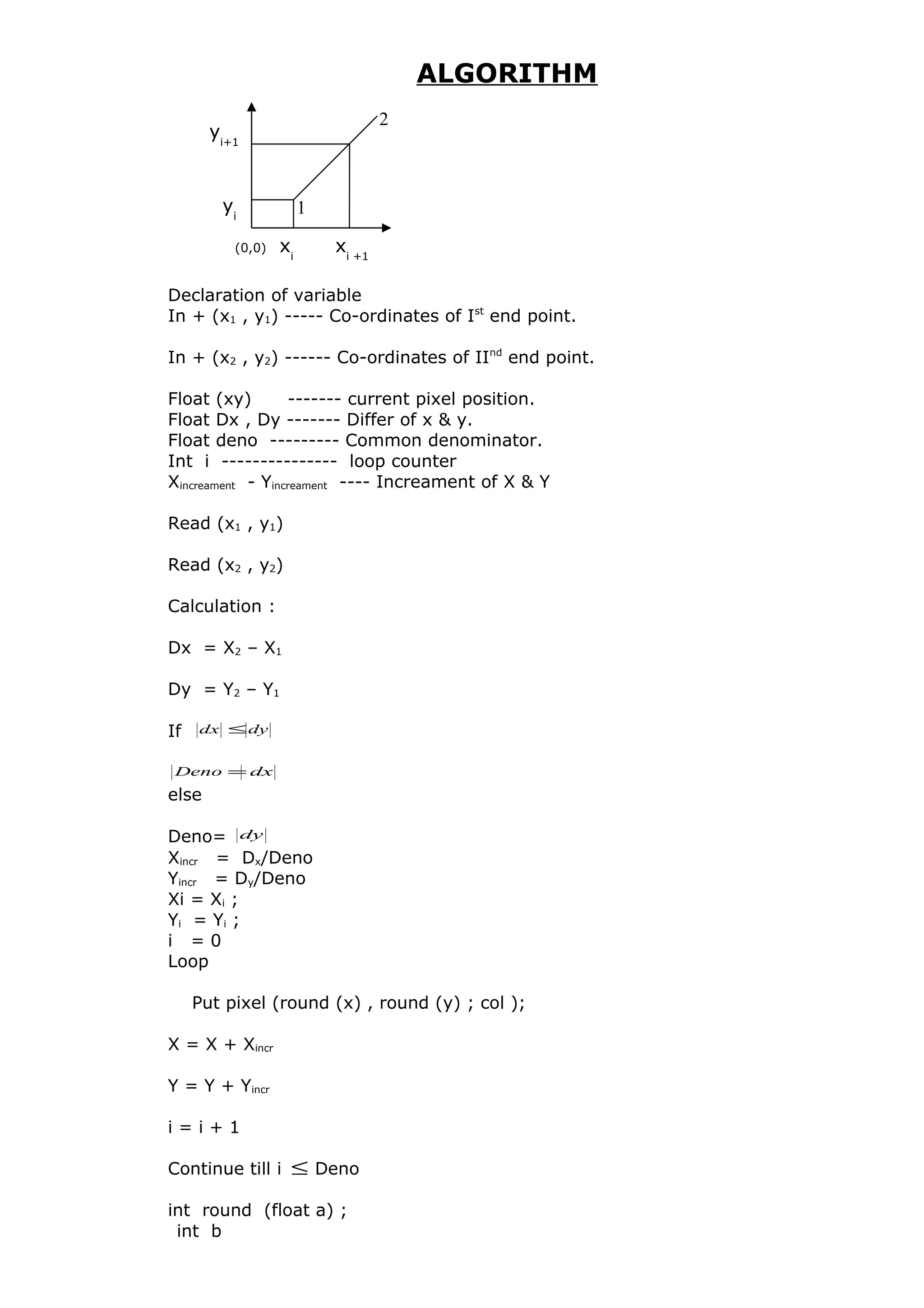
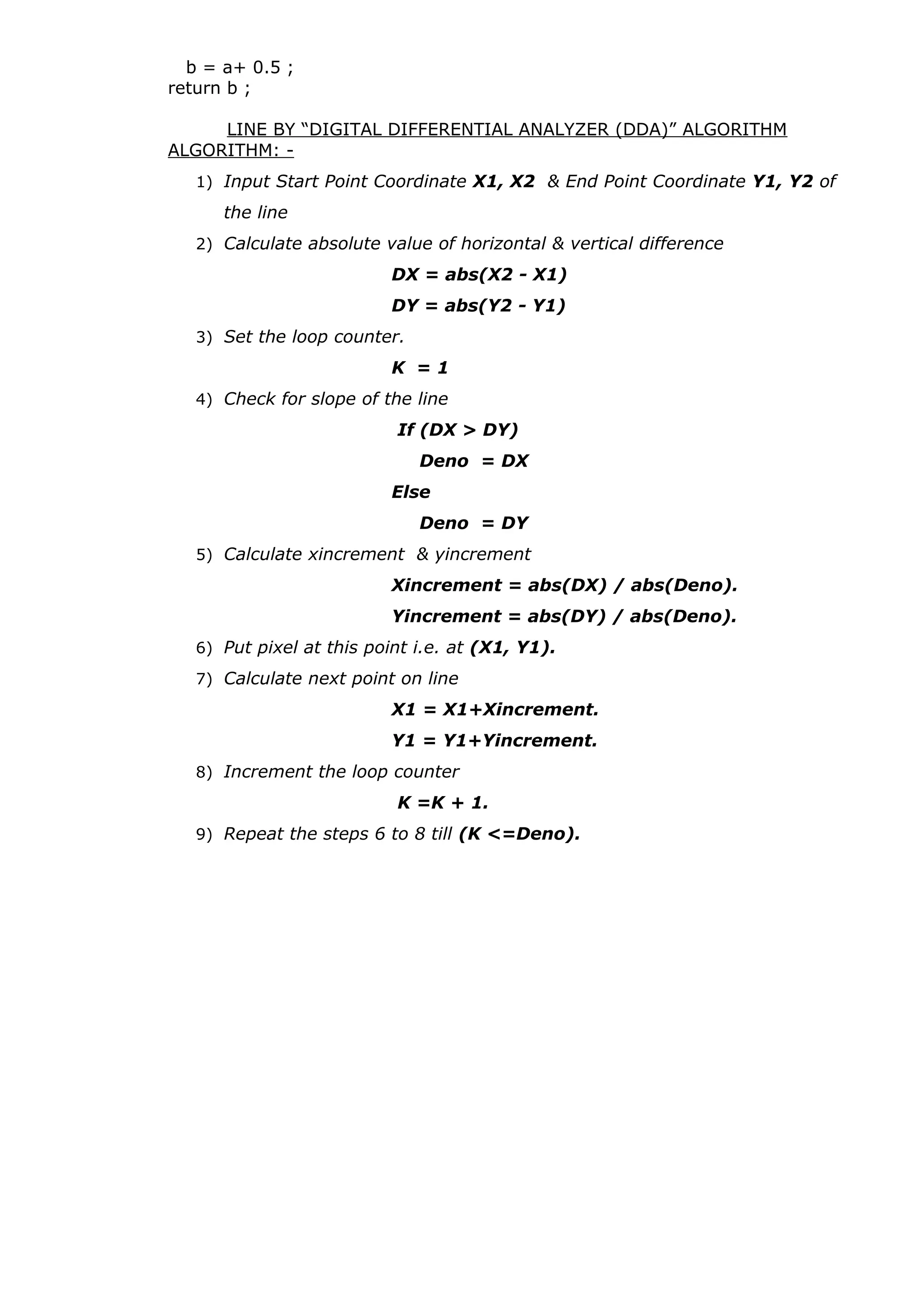
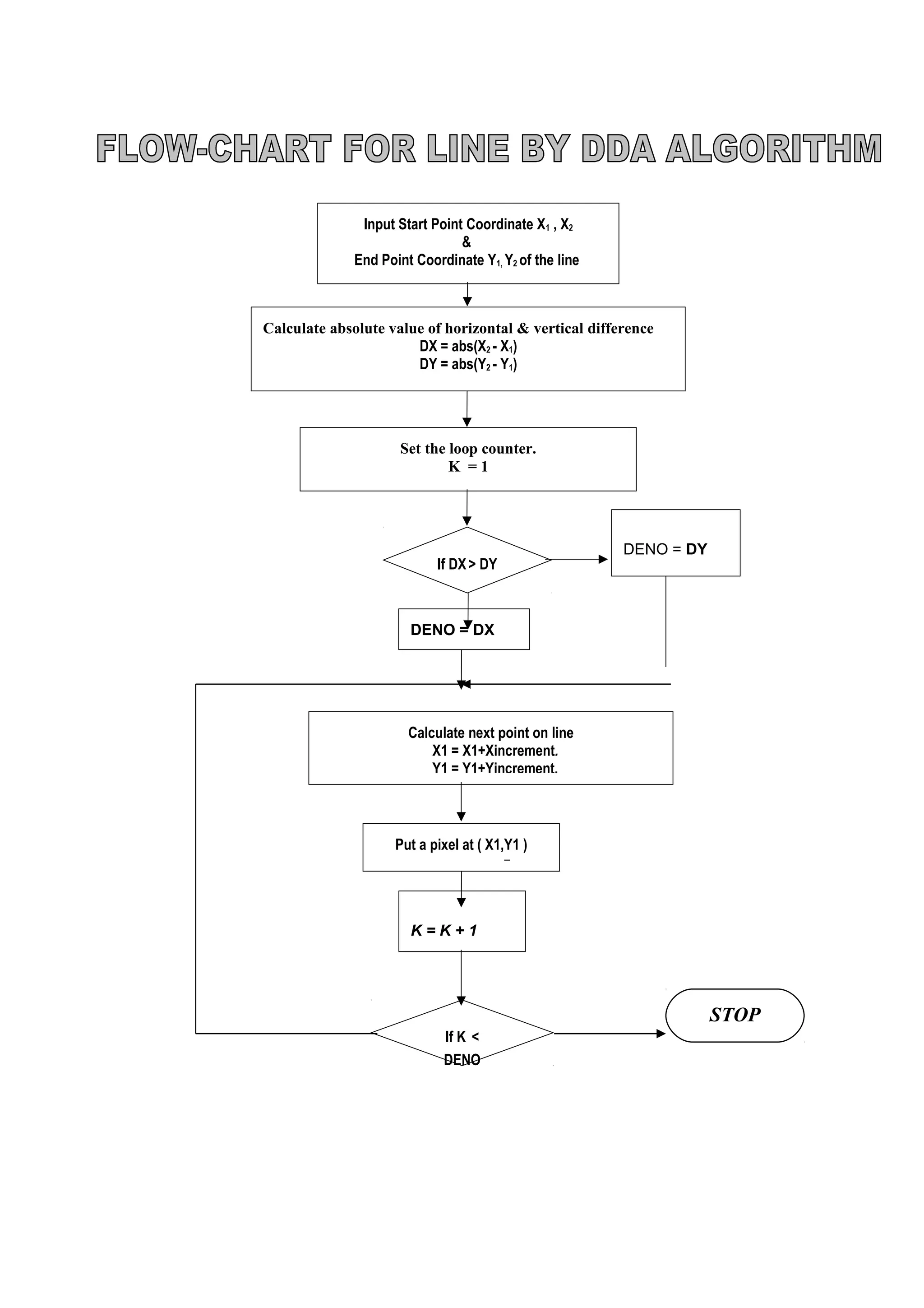
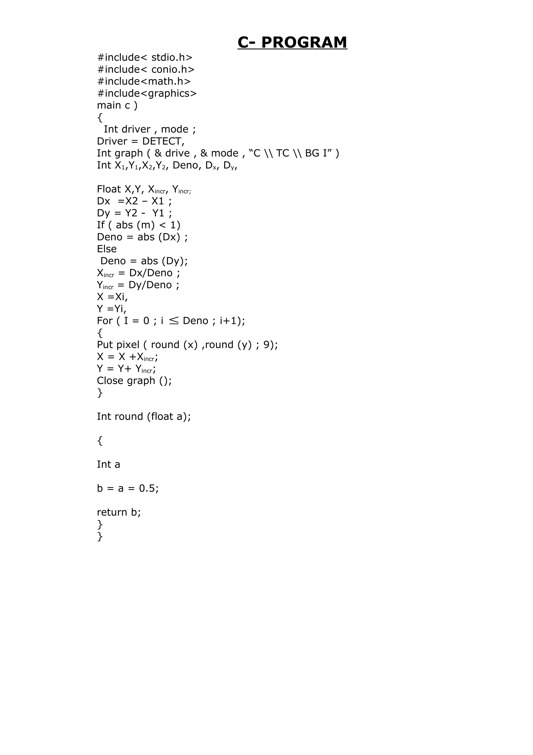
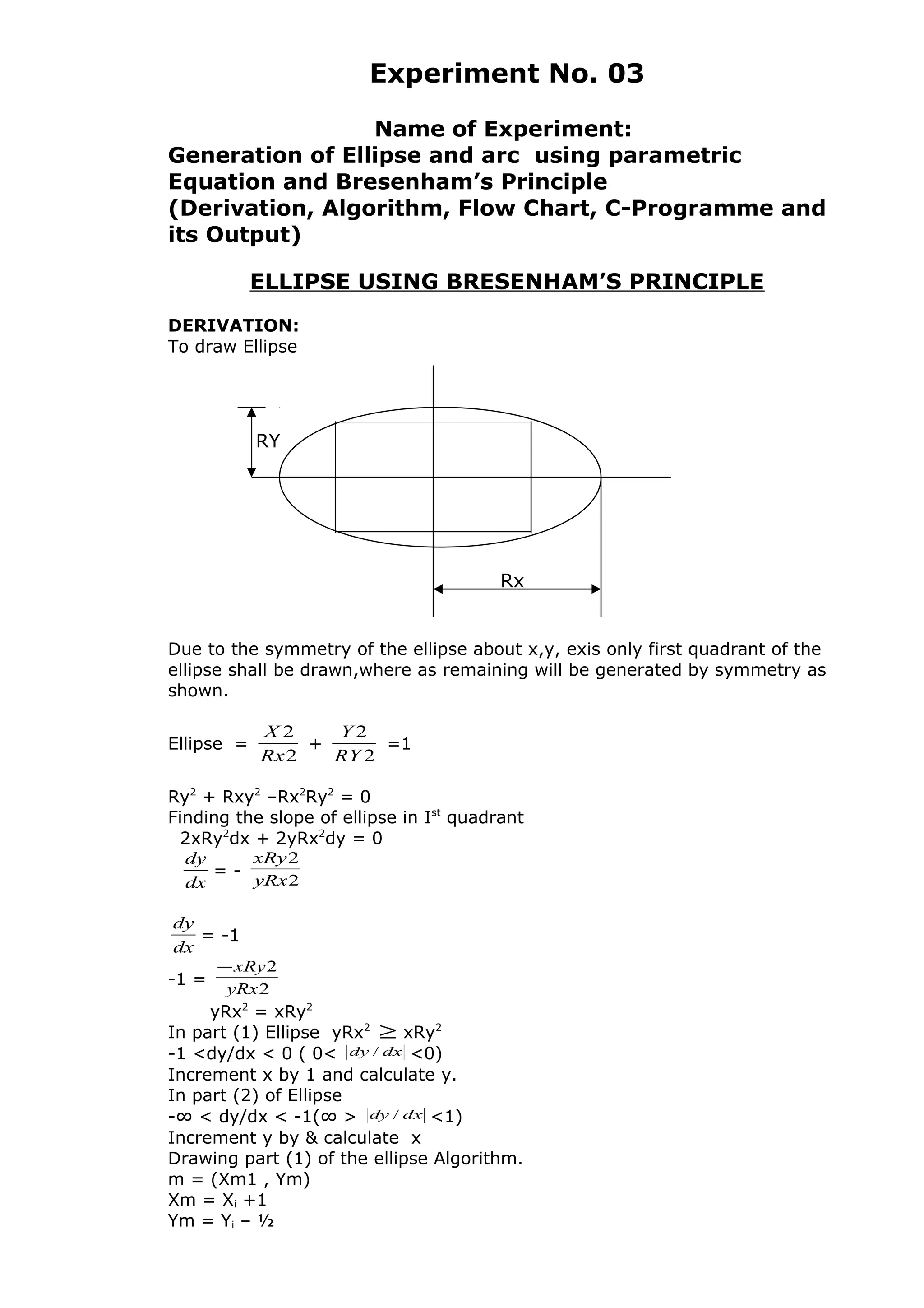
ALGORITHM
1) Declaration of variables:
Int (Xc,Yc)- Co-ordinate of Centre of circle
Int R – Radius of Circle](https://image.slidesharecdn.com/camdpractical-150318103014-conversion-gate01/75/Computer-Aided-Manufacturing-Design-21-2048.jpg)


![EQUATION OF CIRCLE:
SUB CO-ORDINATE OF MID POINT
Pi = X +Y -
If PI < 0
Xi +1 = Xi +1
Yi = Y
Else Pi > 0
Xi +1 = Xi +Y
Yi = 1
Pi = + -
+ 2Xi + 1 + - Yi + ¼ -
Pi = + 2Xi + 1 + - Yi + [ 1+ ¼ - ]
Pi = + 2Xi + 1 + - Yi + K
Decision base variable k
Pi+1 = + 2 + ( ) – + K
Pi +1 – P1 = - ( ] + 2(Xi+1 - Xi)+ – ] + ( Yi+1 - Yi )
Pi+1 = Pi + - ( ] + 2(Xi+1 - Xi)+ – ] + ( Yi+1 - Yi )
If Pi < 0
=](https://image.slidesharecdn.com/camdpractical-150318103014-conversion-gate01/75/Computer-Aided-Manufacturing-Design-27-2048.jpg)
![Decision Variable
Pi = Ry2
x2
+ Rx2
y2
– Rx2
Ry2
Pi = Ry2
xm2
+ Rx2
Ym2
- Rx2
y2
Pi =Ry2
(Xi +1)2
+ Rx2
(Yi – ½)2
- Rx2
Ry2
Pi =Ry2
(Xi
2
+ 2Xi +2) + Rx2
(Yi
2
– Yi +1/4) – Rx2 Ry2
Pi =Ry2
(Xi
2
+ 2Xi ) + Rx2
(Yi
2
– Yi ) + [Ry2
+1 +
4
2Rx
- Rx2
Ry2
]
Pi =Ry2
(Xi
2
+ 2Xi ) + Rx2
(Yi
2
– Yi ) +K-------I
Where K= Ry2
+1 +
4
2Rx
- Rx2
Ry2
+1
Pi+1 = Ry2
( Xi+1
2
+2 Xi+1) + Rx2
(Yi+1
2
- Yi+1) +K---II
Sub Equation II & I
Pi+1 = Pi+ Ry2
{( Xi+1
2
- Xi
2
) + 2(Xi+1 - Xi)}
+ Rx2
{(Yi+1
2
- Yi
2
) – (Yi+1- Yi)}
If Pi 0≤ (midpoint inside)
Xi+1 = Xi+1
Yi+1 = Yi
Pi+1 = Pi+ Ry2
{( Xi+1
2
- Xi
2
) + 2(Xi+1 - Xi)}
+ Rx2
{(Yi
2
- Yi
2
) – (Yi- Yi)}
=Pi+ Ry2
{( Xi
2
+ 2Xi +1) +2}+ Rx2
{0}
Pi+1 = Pi+ Ry2
(2Xi +3)
If Pi > 0 (midpoint outside)
Xi+1 = Xi+1
Yi+1 = Yi-1
Pi+1 =Pi+ Ry2
{( Xi+1
2
- Xi
2
)+2(Xi+1 - Xi)}+Rx2
{( Yi-1)2
- Yi
2
]-[ Yi -1- Yi]
=Pi+ Ry2
{( Xi
2
+ 2Xi +1) +2}+ Rx2
{ Yi
2
-2Yi+1- Yi
2
]-[-1]
Pi+1 =Pi+ Ry2
[2Xi +3]+ Rx2
[-2Yi+2]
First Decision Variable
Xi = 0; Yi=Ry
Substitute in Equation I
Pi= Ry2
(Xi
2
+ 2Xi) + Rx2
(Yi
2
- Yi)+ Ry2
4
2Rx
-Rx2
-Rx2
Ry2
= Ry2
(0) + Rx2
(Ry2
- Ry)+ Ry2
+
4
2Rx
- Rx2
Ry2
=Rx2
Ry2
- Rx2
Ry+ Ry2
+
4
2Rx
- Rx2
Ry2
= Ry2
- Rx2
(Ry-1/4)
P ≈ Ry2
- Rx2
Ry2
ALGORITHM
1) Declaration of Variable
Int (Xc
,Yc
) --- centre of ellipse
Int (x,y) ----Current position of x&y
(0,0) xi
xi +1
R
0,0
Outside Point
Mid point m (Xm
,Ym
) = (Xi+1
,Yi
– ½)
Inside Point
1
2
1-Slope less than 1
2-Slope greater than 1](https://image.slidesharecdn.com/camdpractical-150318103014-conversion-gate01/75/Computer-Aided-Manufacturing-Design-32-2048.jpg)
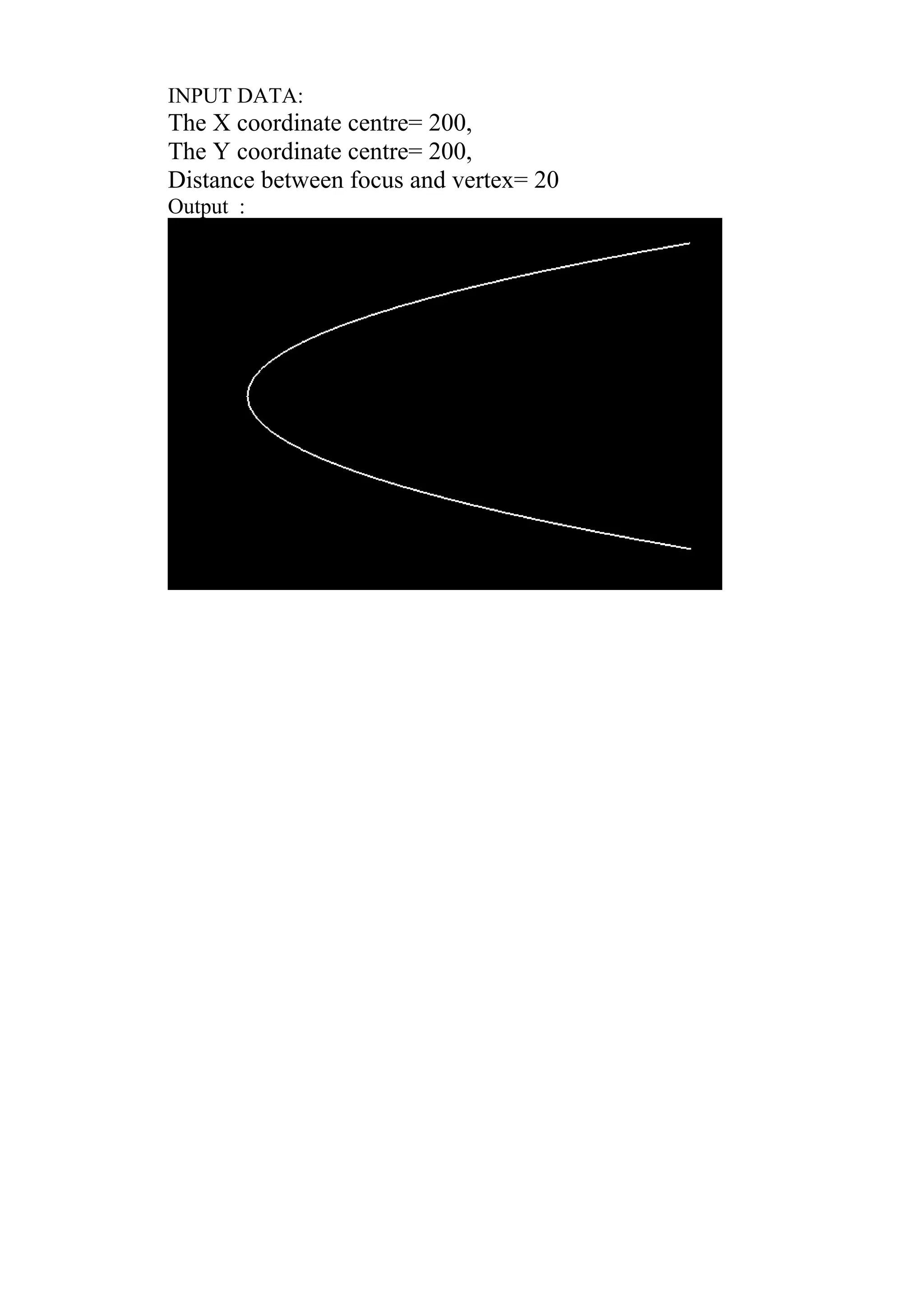
![Derivation of hyperbola
xy = k
dy = -k
dx x^2
-k = -k
x^2
x^2= k
-1< dy < 0
dx
xm= xi +1
ym= yi – y2 xy-x=0
P1 = xm ym = k= 0
P1 = (xi +1) (yi – y) ------------ 1
= xi yi - xi + yi - y2 – k
2
Pi+1 = xi +1, yi + 1- xi +1 + yi + 1 l/2 - k ---------- II
Pi+1 = [(xi +1, yi + 1)- xi yi ] –l/2 [xi +1- xi] + [(yi + 1- yi )]
= RY^2 (xi^2 +2xi + 1) + Rx^2 (yi^2 - yi +l/2 )- Rx^2 Ry^2
= RY^2 (xi^2 +2xi) + Rx^2 (yi^2 - yi)- (Ry^2 Rx^2-Rx^2 Ry^2)
4
Pi = RY^2 (xi^2 +2xi) + Rx^2 (yi^2 - yi)+k ----- I
Pi = RY^2 [ (xi+1 )^2 +2(xi +1)]+ Rx^2[ (yi+1)- yi+1]+k------ II
Pi+1 = Pi+ RY^2[(xi+1 )^2- xi ]+ 2 Rx^2[xi+1 - xi]+ Rx^2[ (yi^2+ yi^2)– (yi+1 - yi)]
If P< 0
xi+1 =xi+1
yi+1 - yi-1
Pi+1 = Pi+ RY^2[(2x+3) ]
If P> 0
xi+1 =xi+1
yi+1 = yi-1
Pi+1 = Pi+ RY^2[(2x+3) ]+ Rx^2[(-xy+2) ]
For first point on hyperbola
xi+ -0
yi= R
P= RY^2[(xi+1 )^2 ]+ 2 Rx^2[yi- l/2]-Rx^2 RY^2
xi+1 =xi+1
yi+1 = yi
Pi+1 = Pi+ [(xi+1 ) yi - xi yi ]-l/2 [xi+1 - xi]+ [ (yi- yi)]
= Pi+ [(xiyi + yi - x yi]- l/2
Pi+1 = Pi+ xi yi –l
If P> 0
xi+1 =xi+1](https://image.slidesharecdn.com/camdpractical-150318103014-conversion-gate01/75/Computer-Aided-Manufacturing-Design-43-2048.jpg)


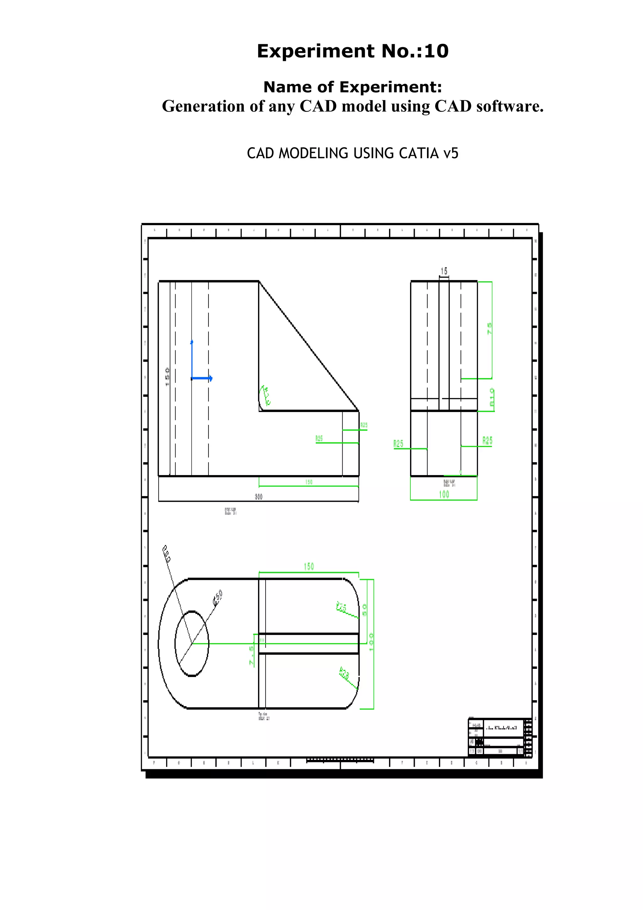
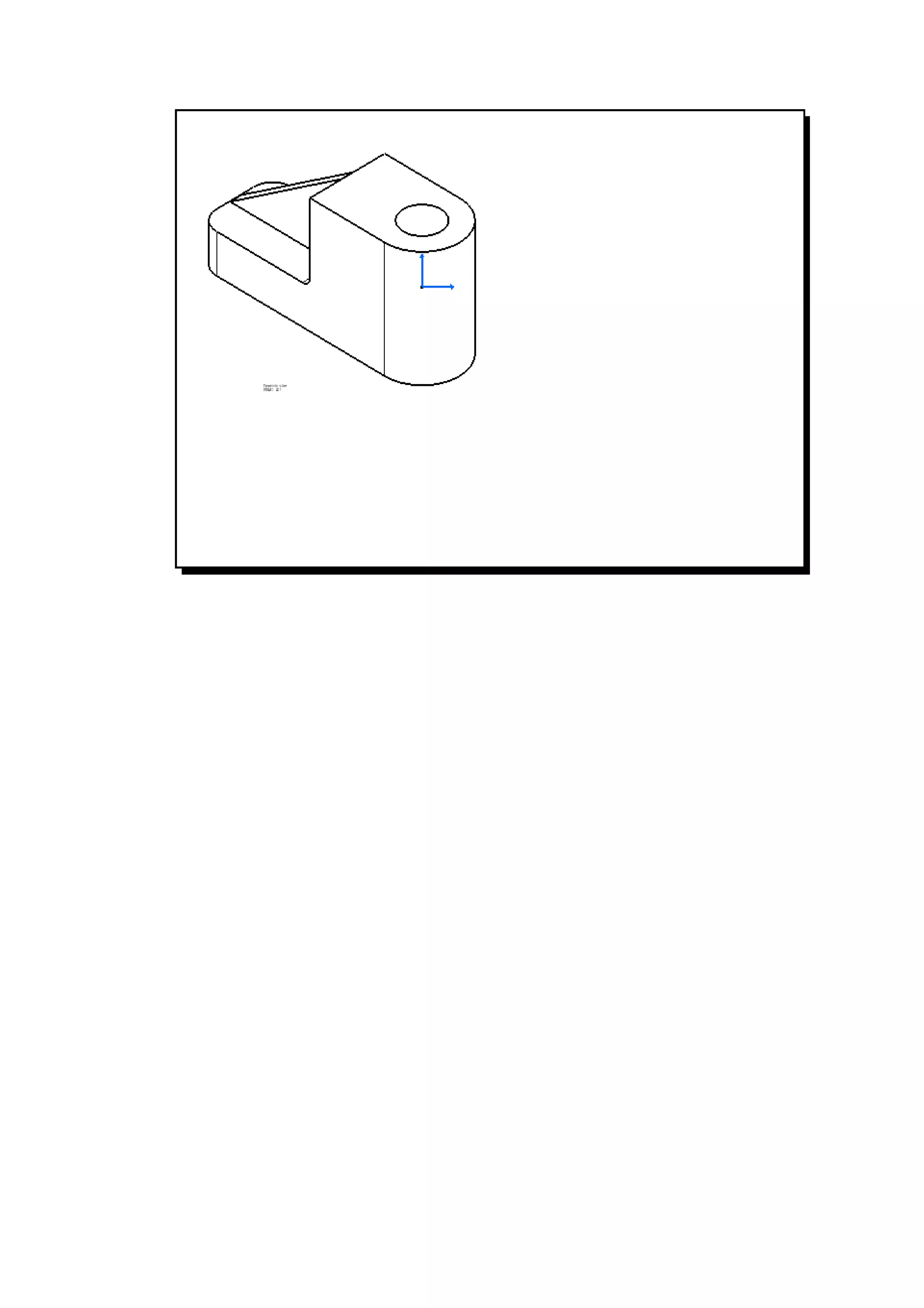
![Experiment No.:06
Name of Experiment:
Generation of Synthetic Curves (Bezier and B-Spline)
ALGORITHM FOR B-SPLINE CURVES
ALGORITHM: -
1) Initialization of all the required parameters.
2) Enter the co-ordinates of four control point Px(4) and Py(4).
3) For four control points degree (n) is three.
4) Calculate the knot vector as:
0 j<k
Uj = j-k+1 k j n
n-k+2 j>n
where,
0 j n +k
for the range of u,
0 u n – k + 2
5) Calculate the B-spline function for the four control points as
Ni,k(u) = (u-uj) Ni,k-1(u)/(ui,k+1-ui) + (ui+k-u) Ni+1,k-1(u)/(ui+k-ui-1)
Where,
Ni,j = 1, ui u ui+1
O, otherwise
Considering 0/0 = 0 if the denominator in above equation becomes
zero
6) Calculate the corresponding four control points on the B-Spline curve as
P(u)x = Px[0]*N0,4+Px[1]*N1,4+Px[2]*N2,4+Px[3]*N3,4 for 0 u 1
P(u)y = Py[0]*N0,4+Py[1]*N1,4+Py[2]*N2,4+Py[3]*N3,4 for 0 u 1
By incrementing u in small step.
7) Graphics Initilisation.
8) Plot the co-ordinates](https://image.slidesharecdn.com/camdpractical-150318103014-conversion-gate01/75/Computer-Aided-Manufacturing-Design-52-2048.jpg)
![/* Program for "B-Spline" */
#include<math.h>
#include<graphics.h>
#include<stdlib.h>
#include<stdio.h>
#include<conio.h>
void main(void)
{
int i,j,n,m,m1,k,x,s,k1;
float Umax,Umin,u,Uk[10],N[20][20],px[4],py[4]={0},X[4]={0},Y[4]={0};
float num1=0,num2=0,deno1=0,deno2=0,Ax[4]={0},Ay[4]={0},sumX=0,sumY=0;
int gdriver = DETECT, gmode, errorcode;
clrscr();
printf("nEnter the number of control point ");
scanf("%d",&k);
printf("nEnter the coordinate of control point ");
for(i=0;i<=k-1;i++)
{
scanf("%f",&px[i]);
scanf("%f",&py[i]);
}
k1=k;
n=k-1;
Umin=0;
Umax=n-k+2;
s=n+k;
for(j=0;j<=n+k;j++)
{
if(j<k)
Uk[j]=0;
else
{
if(j>=k&&j<=n)
Uk[j]=j-k+1;
else
{
if(j>n)
Uk[j]=n-k+2;
}
}
}
for(i=0;i<=n;i++)
{
for(k=1;k<=n;k++)
{
if((i+k)>s)
continue;
else
{
if(Uk[i+k-1]-Uk[i]==0&&Uk[i+k]-Uk[i+1]==0)
{
N[i][k]=0;
}
}
}
}
for(i=0;i<=n;i++)
{
if(u>=Uk[i]||u<=Uk[i+1])
N[i][1]=1;
else
N[i][1]=0;
}](https://image.slidesharecdn.com/camdpractical-150318103014-conversion-gate01/75/Computer-Aided-Manufacturing-Design-53-2048.jpg)
![initgraph(&gdriver, &gmode, "");
errorcode = graphresult();
if (errorcode != grOk) /* an error occurred */
{
printf("Graphics error: %sn", grapherrormsg(errorcode));
printf("Press any key to halt:");
getch();
exit(1); /* terminate with an error code */
}
for(u=0;u<=1;u=u+0.01)
{
for(k=2;k<=(n+k)-1;i++)
{
for(i=0;i<=(n+k)-1;i++)
{if((i+k)>s)
break;
else
{
x=i+k-1;
deno1=(Uk[x]-Uk[i]);
deno2=(Uk[i+k]-Uk[i+1]);
num1=((u-Uk[i])*(N[i][k-1]));
num2=((Uk[i+k]-u)*(N[i+1][k-1]));
if(deno1==0)
{num1=0;
}
if(deno2==0)
{
num2=0;
}
N[i][k]=(num1/deno1)+(num2/deno2);
}
}
}
for(m1=0;m1<4;m1++)
{
Ax[m1]=px[m1]*N[m1][k1];
Ay[m1]=py[m1]*N[m1][k1];
sumX=sumX+Ax[m1];
sumY=sumY+Ay[m1];
}
putpixel(50*sumX,50*sumY,3);
sumX=0;
sumY=0;
}
getch();
closegraph();
getch();
}](https://image.slidesharecdn.com/camdpractical-150318103014-conversion-gate01/75/Computer-Aided-Manufacturing-Design-54-2048.jpg)

![Experiment No.:07
Name of Experiment:
Two Dimensional Transformation (Any Two Numerical)
Q.1: A triangle with vertices at A(0,0),B(8,0),C(0,8) is scaled by
1.2 units in X direction. It is translated by 3.5 units in Y direction
and two units X direction. Find the final position of the triangle.
Show the total transformation on graph paper stepwise.
Ans. The original position of the given ∆ ABC is shown in graph paper.
The final transformation is given as,
P’ = P.TT
Where TT = Total transformation
TT = S.T.
P =
180
108
100
S =
100
00
00
Sy
Sx
=
100
010
002.1
T =
0
010
001
tytx
T =
15.32
010
001
TT = [ ]S X [ ]T
=
100
010
002.1
.
15.32
010
001
TT =
15.30
010
002.1
P’ = [ ]P .[ TT]
=
180
108
100
15.32
010
002.1](https://image.slidesharecdn.com/camdpractical-150318103014-conversion-gate01/75/Computer-Aided-Manufacturing-Design-56-2048.jpg)
![P’ =
15.112
15.36.11
15.32
The final position of triangle ABC is shown on graph paper.
Coordinates of ∆ A’B’C are;
A’ (2,3.5)
B’ (11.6,3.5)
C’ (2,11.5)
Q.2: Find the transformation which converts the fig. defined by
vertices
A(3,2),B(2,1) and C(4,1) into another figure which is defined by
Vertices A’(-3,-1),B(-4,-2) and C’(-2,-2).
Ans. Let [P’] – is final position of triangle A’B’C’
[P] - is initial position of triangle ABC
[G] – is transformation matrix.
Given data:
Final position of triangle is
A’(-3,-1)
B’(-4,-2)
C’(-2,-2)
Initial position of triangle is
A(3,2)
B(2,1)
C(4,1)
General expression for determining final position of object is
[P’] = [P] [G]
∴[G] = [P]-1
[P’]……………………………….(1)
Now
Final position [P’] =
−−
−−
−−
122
124
113
And initial position
[P]=
114
112
123
Inverse matrix [P] is given by following generalized equation
[P]-1
=
]det[
][int
P
PofAdjo
……………………….(2)](https://image.slidesharecdn.com/camdpractical-150318103014-conversion-gate01/75/Computer-Aided-Manufacturing-Design-57-2048.jpg)
![Co-factor of [P] = -
12
23
14
23
14
12
12
13
14
13
14
12
11
12
11
12
11
11
−
−
=
−−
−−
−
111
511
220
When rows are converted into columns. Adjoint of [P] is determined
∴Adj[P] =
−−
−−
−
111
511
220
Similarly determinant of [P] is determined as det [P] = 3(1-1)-2(2-4)+(2-
4)
= 2
From equation (2)
[P]-1
=
]det[
][int
P
PofAdjo
=
−−
−−
−
2
1
2
5
1
2
1
2
1
1
2
1
2
1
0
Thus, substituting values of [P]-1
in equation (1)
[G] =
−−
−−
−
2
1
2
5
1
2
1
2
1
1
2
1
2
1
0
−−
−−
−−
122
124
113
∴[G] =
−− 136
010
001
Check
[P’] = [P] [G]
=
114
112
123
−− 136
010
001](https://image.slidesharecdn.com/camdpractical-150318103014-conversion-gate01/75/Computer-Aided-Manufacturing-Design-58-2048.jpg)
![Experiment No.:08
Name of Experiment:
Three Dimensional Transformation (Any Two Numerical)
Q.1: Consider a region defined by the position vectors
[ ]X =
1221
1222
1212
1211
D
C
B
A
Relative to the global XYZ axis system. It is rotated by +300
about the X’ axis parallel to X axis and passing through point
(1.5,1.5,1.5,1).Find the final transformation matrix and final
positions of the region.
Ans. The final transformation is carried out as follows.
[ ]'X =
1221
1222
1212
1211
4x4
Steps : (1) We will first translate the object so that rotation axis X’
coincide with the X axis.
(2) Perform rotation about the object so that 300
ccw, (θ = +300
)
(3) Again translate the object so that X’ moves to its original position.
∴ T1 =
1111
0100
0010
0001
tztytx
4x4
tx1 = -1.5, ty1 = -1.5, tz1 = -1.5
T1 =
−−− 15.15.15.1
0100
0010
0001
4x4
∴ Rx =
°°−
°°
1000
030cos30sin0
030sin30cos0
0001
4x4
∴ Rx =
−
1000
0866.05.0
05.866.00
0001
4x4](https://image.slidesharecdn.com/camdpractical-150318103014-conversion-gate01/75/Computer-Aided-Manufacturing-Design-64-2048.jpg)
![T2 =
15.15.15.1
0100
0010
0001
4x4
∴ TT = [T1].[ Rx].[T2]
=
−−− 15.15.15.1
0100
0010
0001
x
−
1000
0866.05.0
05.866.00
0001
x
15.15.15.1
0100
0010
0001
∴ TT =
−−−
−
1049.2549.05.1
0866.05.00
05.866.00
0001
15.15.15.1
0100
0010
0001
TT =
−
−
1549.0951.00
0866.05.00
05.0866.00
0001
…..Final Transformation Matrix
4x4
Now we will find final positions of the region.
X’ = [X] [TT]
=
1221
1222
1212
1211
−
−
1549.0951.00
0866.05.00
05.0866.00
0001
4x4 4x4
X’ =
1183.2683.11
1183.2683.12
1683.1817.02
1683.1817.01
4x4
Numerical for Practical:
1. Determine the 4 X 4 transformation matrices for the rotation of 3-D
point in 3-D space.](https://image.slidesharecdn.com/camdpractical-150318103014-conversion-gate01/75/Computer-Aided-Manufacturing-Design-65-2048.jpg)

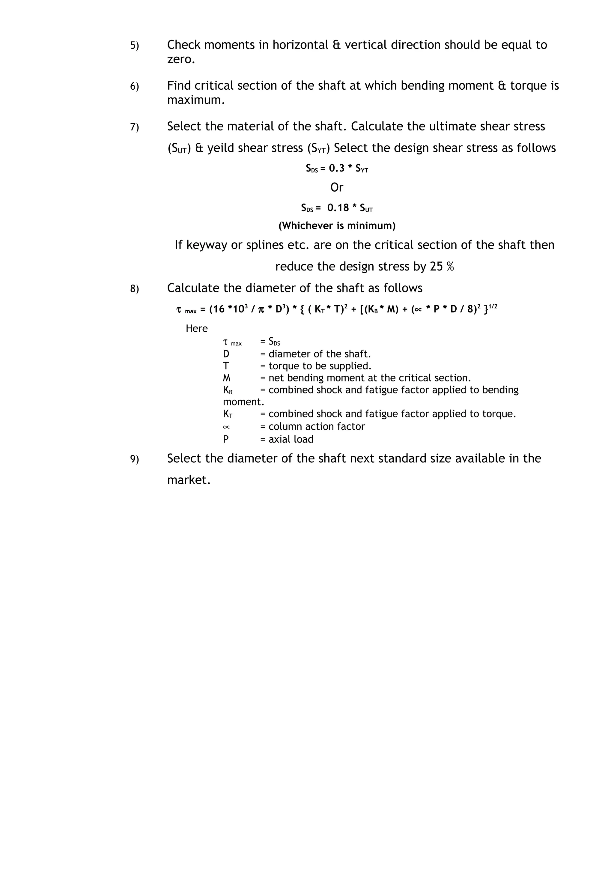
![/* PROGRAM OF DESIGN OF SHAFT */
#include<stdio.h>
#include<math.h>
#include<stdlib.h>
#include<string.h>
#include<conio.h>
#include<dos.h>
#define PI 3.141592654
#define max_matls 13
#define max_input 4
void main()
{
float Reaction(float,float,float,float,float);
float Diameter(long,long,float,float);
char matl[max_matls][15],matl_in[max_matls][15];
long T,P,M,Me,Te,x;
int i,j,Syt[max_matls]={0},Sut[max_matls]={0},Rho[max_matls]={0};
float Ss,Sd,Ss1,Sd1,x1,x2;
float l,l1,l2,l3,d,d1,d2,d3,d4,Km,Kt,RA,RD,WB,WC,MB,MC,N;
FILE*fp;
clrscr();
fflush(stdin);
printf("nEnter Power[W] : ");
scanf("%ld",&P);
printf("nEnter Speed of The Shaft [RPM] : ");
scanf("%f",&N);
printf("nEnter distance between Bearing and Gear [mm] : ");
scanf("%f",&l1);
printf("nEnter distance between Gear and Pulley [mm] : ");
scanf("%f",&l2);
printf("nEnter distance between Pulley and End Bearing [mm] : ");
scanf("%f",&l3);
printf("Enter the Load Acting on Gear [N] : ");
scanf("%f",&WB);
printf("Enter the Load Acting on Pulley [N] : ");
scanf("%f",&WC);
RD=Reaction(WB,WC,l1,l2,l3);
RA=WB+WC-RD;
MB=RD*(l2+l3);
MC=RD*l3;
if(MB>MC)
M=MB;
else
M=MC;
T=P*60/(2*PI*N);
printf("Enter Combined shock & Fatiuge Factor for Bending : ");
scanf("%f",&Km);
printf("Enter Combined shock & Fatiuge Factor for Torsion : ");
scanf("%f",&Kt);
x=(Km*M*Km*M)+(Kt*T*Kt*T);
Te=sqrt(x);
Me=0.5*(M+Te);
if((fp=fopen("sd1.dat","r"))==NULL)
{
printf("Unable to Openn");
printf("Sorry!!! Please Try Again");
getch();
exit(0);
}
else](https://image.slidesharecdn.com/camdpractical-150318103014-conversion-gate01/75/Computer-Aided-Manufacturing-Design-69-2048.jpg)
![{
printf("nfile opened successfully!");
printf("nMaterialtSyttDensity");
for (i=0;i<=max_matls-1;i++)
{
fscanf(fp,"%s%d%d",&matl[i],&Syt[i],&Rho[i]);
printf("n%stt%dt%d",matl[i],Syt[i],Rho[i]);
}
for (i=0;i<=0;i++)
{
printf("nEnter Material No : ");
scanf("%s",&matl_in[i]);
for (j=0;j<=max_matls-1;j++)
{
if ((strcmp(matl_in[i],matl[j]))==0)
{
Ss=Syt[j]/2;
Sd=0.3*Syt[j];
break;
}
else
continue;
}
}
d=Diameter(Te,Me,Ss,Sd);
if(MB>MC)
{
d1=d;
d2=d+3;
d3=d2+3;
d4=d-5;
Ss1=(T*16)/(PI*d4*d4*d4);
if(Ss1<Ss)
printf("nDesign is Safe");
else
printf("Diameter for the Bearing Allocation is to be redesigned");
}
else
{
d2=d;
d1=d-3;
d3=d2+3;
d4=d-5;
Ss1=(T*16)/(PI*d1*d1*d1);
Sd1=(M*32)/(PI*d1*d1*d1);
if(Ss1<Ss||Sd1<Sd)
printf("nDesign is Safe");
else
printf("Diameter for the Bearing and Gear Allocation is to be redesigned");
}
printf("n--------------------------------------------------------");
printf("nRESULT: ");
printf("nSelected Material: %s ",matl_in[0]);
printf("Designed Diameters of Stepped Shaft are nd1= %fnd2= %fnd3= %fnd4=
%f",d1,d2,d3,d4);
}
getch();
fcloseall();
}
float Reaction(float WB,float WC,float l1,float l2,float l3)
{
float RD,l;](https://image.slidesharecdn.com/camdpractical-150318103014-conversion-gate01/75/Computer-Aided-Manufacturing-Design-70-2048.jpg)

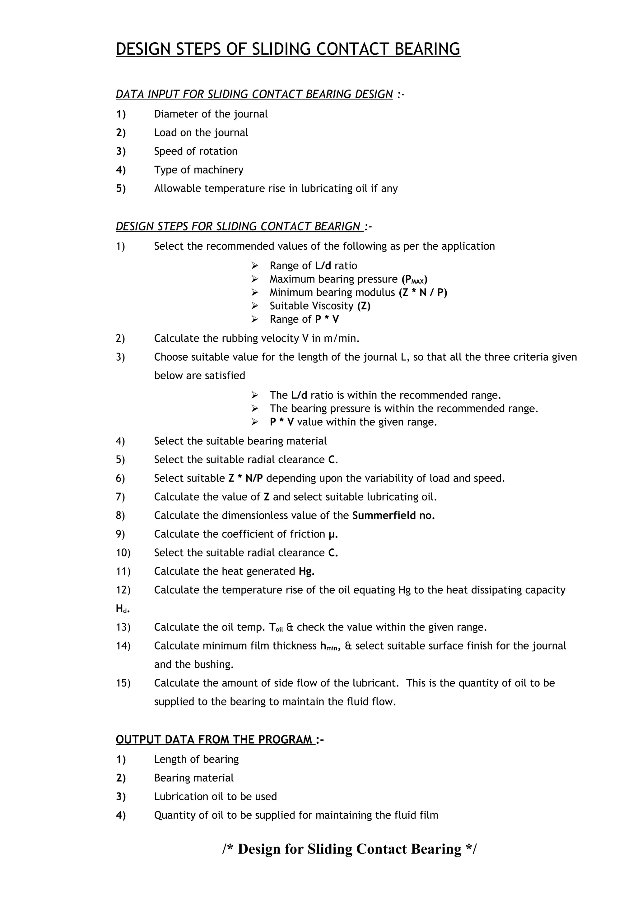
![#include<math.h>
#include<stdlib.h>
#include<stdio.h>
#include<conio.h>
#include<string.h>
#define PI 3.141592654
#define max_matls 5
#define max_input 4
void main()
{
float W,to,Z,ta,pmax,p,t,C,c,l,d,R,Ov,Od,K,cd1,u,k,Hg,Hd,V,A,S,m;
int i,j,N;
char matl[max_matls][25],matl_in[max_matls][25],Mtl;
float
visco[max_matls]={0},cd[max_matls]={0},ld[max_matls]={0},ZN_p[max_matls]={0};
FILE *fp;
clrscr();
fflush(stdin);
printf("nEnter load on journal (Newton) ");
scanf("%f",&W);
printf("nEnter speed of journal(rpm) ");
scanf("%d",&N);
printf("nEnter the ambient temp of oil(deg C) ");
scanf("%f",&ta);
printf("nEnter the maximum pressure of bearing(N/mm2) ");
scanf("%f",&pmax);
/*design starts*/
printf("nEnter the assumed dia of journal(mm) ");
scanf("%f",&d);
if((fp=fopen("Bdata.dat","r"))==NULL)
{
printf("Unable to Openn");
printf("Sorry!!! Please Try Again");
getch();
exit(0);
}
else
{
printf("nFile Opened Successfully!");
printf("nApplicationtViscositytZN/pttc/dtl/d");
for(i=0;i<=max_matls;i++)
{
fscanf(fp,"%s%f%f%f%f",&matl[i],&visco[i],&ZN_p[i],&cd[i],&ld[i]);
printf("n%stt%ft%ft%ft%f",matl[i],visco[i],ZN_p[i],cd[i],ld[i]);
}
for(i=0;i<=0;i++)
{
printf("nEnter Material No,%d : ", i+1);
scanf("%s",&matl_in[i]);
for (j=0;j<=max_matls-1;j++)
{](https://image.slidesharecdn.com/camdpractical-150318103014-conversion-gate01/75/Computer-Aided-Manufacturing-Design-73-2048.jpg)
![if ((strcmp(matl_in[i],matl[j]))==0)
{
l=ld[j]*d;
p=W/(l*d);
Ov=(visco[j]*N)/p;
K=ZN_p[j]/3;
k=0.002; /*for l/d ratio of 0.75 to 2.8*/
u=(33*Ov/cd[j])/(pow(10,8)) +k;
break;
}
else
{
/*printf("nMaterial is not Present In The List");*/
continue;
}
}
}
}
if(p<pmax)
{
printf("nDimension l and d are Safe: ");
}
else
{
printf("n New Dimension of l and d are to be selected: ");
}
printf("nEnter the Operating Temp of Oil(deg C): ");
scanf("%f",&to);
printf("nBearing Modulus at Minimum Point of Friction ");
if(Ov>K)
{
printf("nBearing will Operate at Hydrodynamic Conditions");
}
else
{
printf("n Bearing will have Metal to Metal Contact");
}
V=(3.1428*d*N)/60000;
Hg=u*W*V;
printf("nEnter Heat Dissipation Coefficient from data book: ");
scanf("%f",&C);
A=l*d/(pow(10,6));
Hd=(C*A*(to-ta))/2;
printf("n Heat dissipation Hd= %f J/s",Hd);
printf("n Heat generated Hg= %f J/s",Hg);
printf("n A= %f m2",A);
if(Hg>Hd)
{
printf("nBearing is to be re-design by taking higher operating temperature(to) ");
printf("nor Bearing should be cooled artificially");
printf("nEnter specific heat of oil: ");](https://image.slidesharecdn.com/camdpractical-150318103014-conversion-gate01/75/Computer-Aided-Manufacturing-Design-74-2048.jpg)
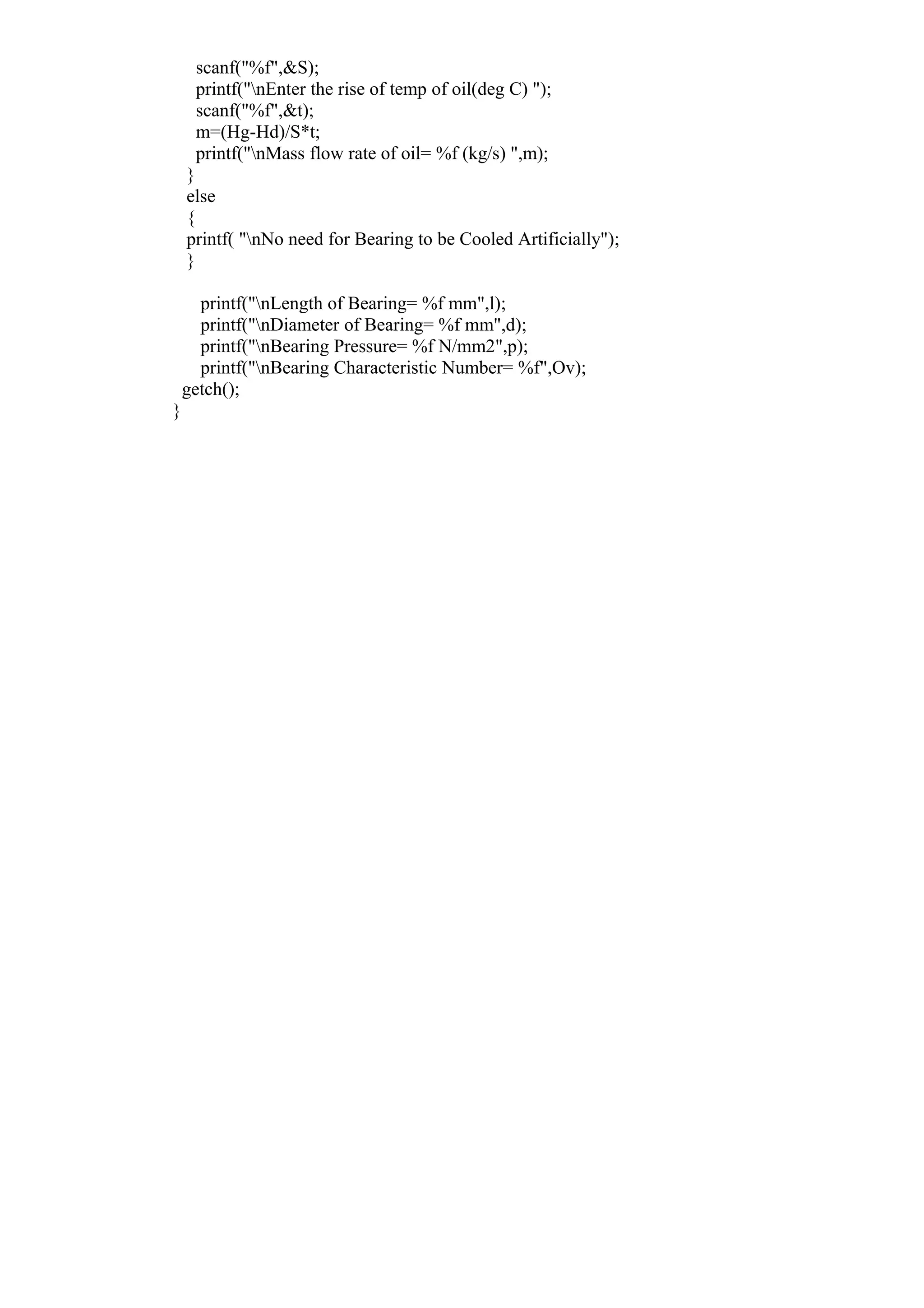
![/* Program to Design Flywheel */
#include<stdio.h>
#include<math.h>
#include<stdlib.h>
#include<string.h>
#include<conio.h>
#include<dos.h>
#define PI 3.141592654
#define max_matls 13
#define max_input 4
void main(void)
{
float m,t,b,rho,FS,Syt,Sd,DE,Cs,D,Rad,k;
char matl[max_matls][15],matl_in[max_matls][15];
float Rho[max_matls]={0};
int syt[max_matls]={0};
int N,i,j;
FILE *fp;
clrscr();
fflush(stdin);
printf("Enter The Speed of the Shaft (RPM) : ");
scanf("%d",&N);
/*printf("Enter the Ultimate Stress in Tension of Material Selected (N/m2) : ");
scanf("%f",&Syt);
printf("Enter the Density of Material Selected (kg/m3) : ");
scanf("%f",&rho);*/
printf("Enter the Factor of Safty For The Material Selected : ");
scanf("%f",&FS);
printf("Enter the Coefficient of Fluctuation of Speed : ");
scanf("%f",&Cs);
printf("Enter the Fluctuation of Energy : ");
scanf("%f",&DE);
if((fp=fopen("sd1.dat","r"))==NULL)
{
printf("Unable to Openn");
printf("Sorry!!! Please Try Again");
getch();
exit(0);
}
else
{
printf("File Opened Successfully!");
printf("nMatl. tsyttrho");
for(i=0;i<=max_matls;i++)
{
fscanf(fp,"%s %d %f",&matl[i],&syt[i],&Rho[i]);
printf("n %s t%dt%f",matl[i],syt[i],Rho[i]);
}
for(i=0;i<=0;i++)
{
printf("nEnter Material No,%d : ", i+1);
scanf("%s",&matl_in[i]);
for(j=0;j<=max_matls-1;j++)
{
if((strcmp(matl_in[i],matl[j]))==0)
{
Syt=syt[j];
Sd=Syt*1000000/FS;
D=(Sd*3600)/(Rho[j]*PI*PI*N*N);
Rad=(2*PI*N)/60;](https://image.slidesharecdn.com/camdpractical-150318103014-conversion-gate01/75/Computer-Aided-Manufacturing-Design-77-2048.jpg)
![m=(4*DE)/(D*D*Rad*Rad*Cs);
k=m/(2*PI*D*Rho[j]*4);
t=sqrt(k);
b=4*t;
break;
}
else
{
/*printf("nMaterial is not Present In The List");
break;*/
continue;
}
}
}
}
clrscr();
printf("You have Selected the Material as %s",matl[0]);
printf("nFor the Entered Data : nDiameter Of The Flywheel is : %f m",D);
printf("nMass of The Flywheel is : %f kg",m);
printf("nThickness of The Flywheel is : %f m",t);
printf("nWidth of The Flywheel is : %f m",b);
getch();
}](https://image.slidesharecdn.com/camdpractical-150318103014-conversion-gate01/75/Computer-Aided-Manufacturing-Design-78-2048.jpg)
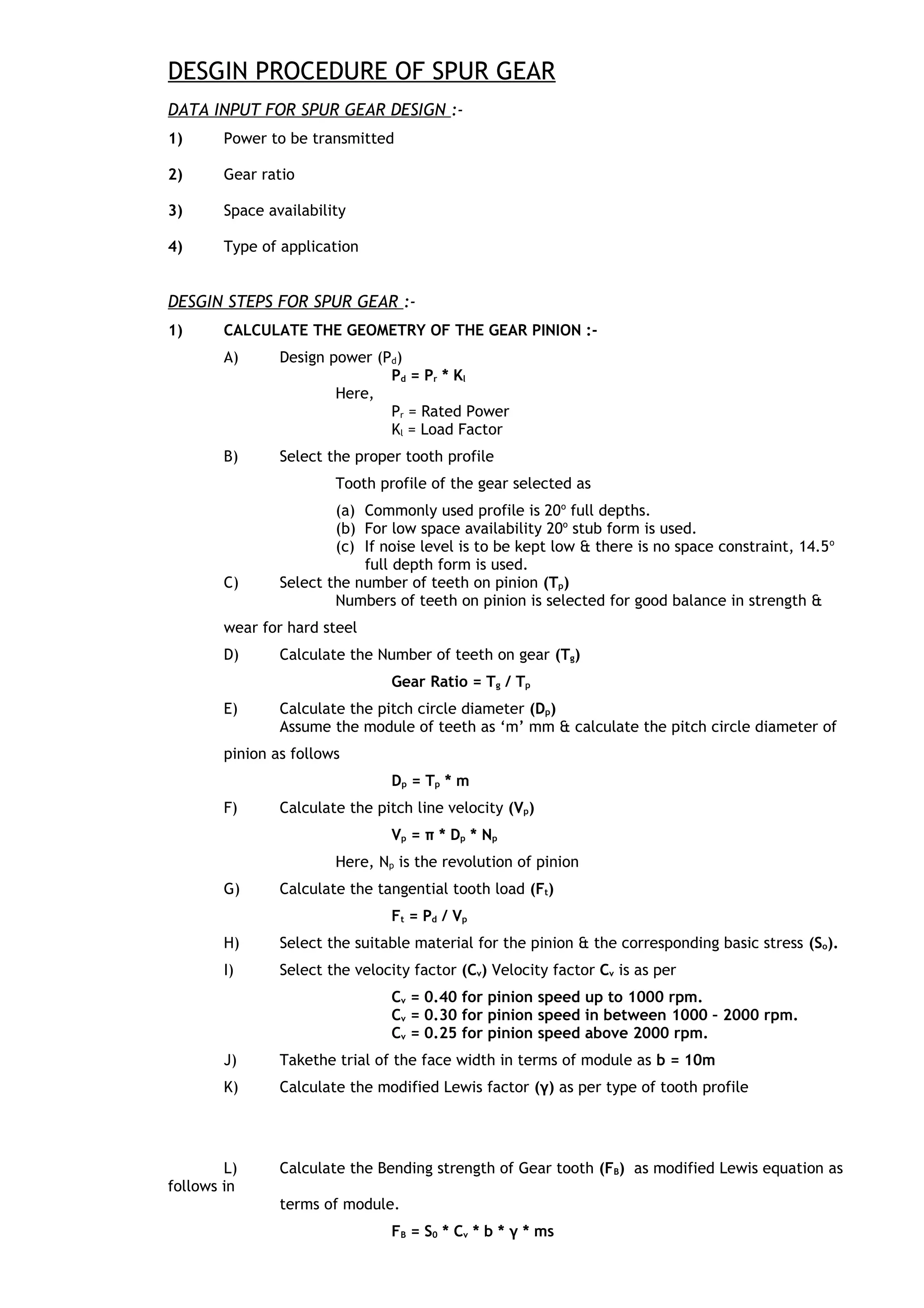
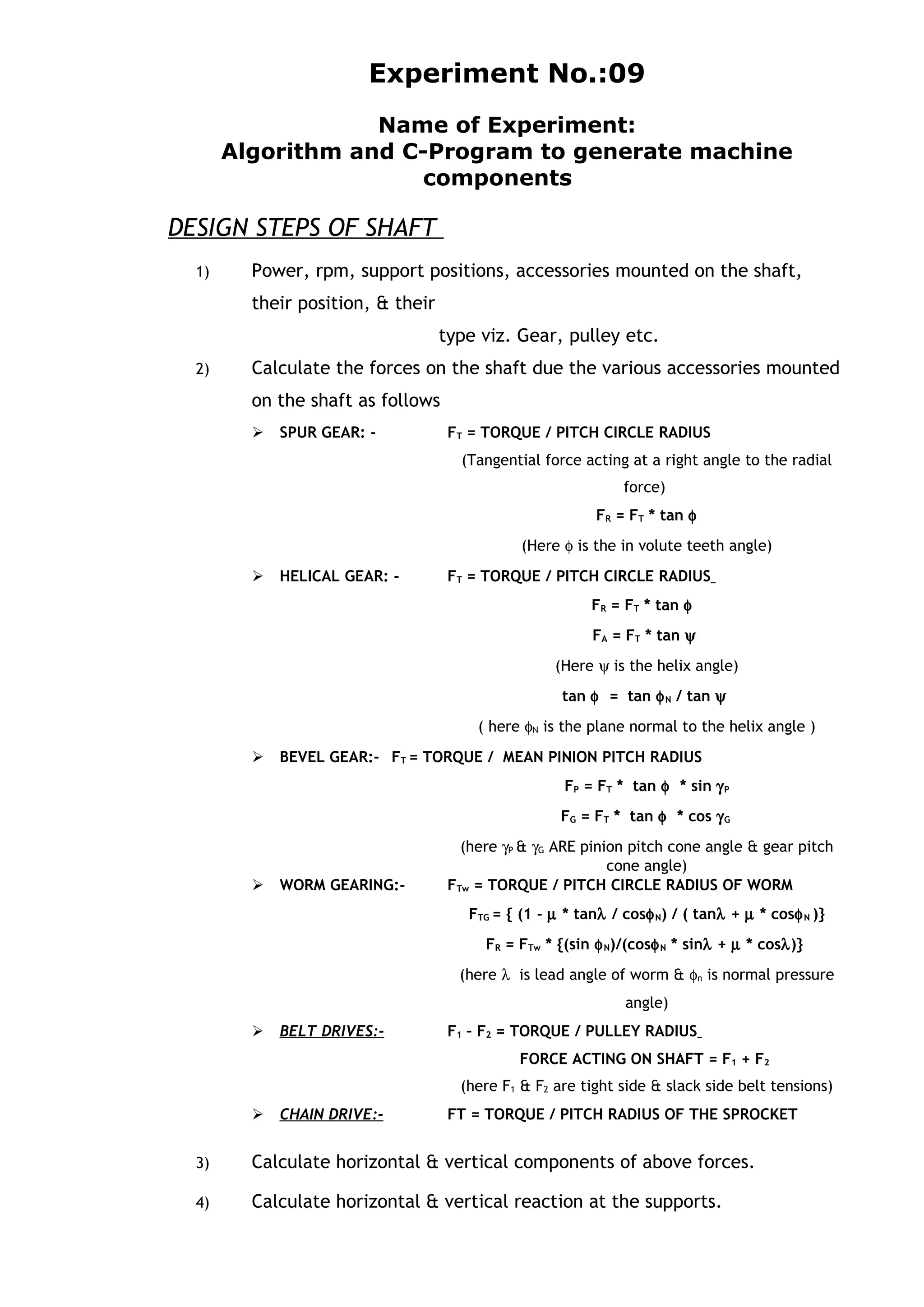
![M) Calculate the module m by equating tangential load FT & bending strength FB
FT = FB
N) Select the next standard module (m) available.
O) Calculate the actual value of Dp with the new module from step N
Dp = 2d + 25 for keyed pinion
Dp = d + 25 for internal pinion
Use the above equation if the shaft diameter is given otherwise
Dp = m * Tp & select Dp such that it should
have higher value.
P) Calculate the actual value of
I. Pitch line velocity (Vp)
II. Velocity fact (Cv)
III. Tangential tooth load (Ft )
IV. Bending strength (FB)
Q) Select the material for the gear & calculate the value of (S0 * γ ) for both pinion
& gear.
R) Take the smaller value of (S0 * γ ) for calculating the face width (b).
S) Calculate face width (b) from the modified Lewis equation.
T) Calculate the face width (minimum) from standard proportion as
b = 8.5 * m
select the bigger value of face width from step S & T
2) DESIGN CHECK FOR DYNAMIC LOAD & LIMITING WEAR STRENGTH.
A) Calculate the dynamic load (Fd)
a) Find out the permissible error in profile as per the pitch line velocity.
b) Decide the class of manufacturing process as the permissible error found
in step a.
c) Find out the probable error in the teeth profile as per module.
d) Calculate the deformation factor “C”. This depends upon the material
of the gear &
pinion along with the type of teeth profile.
Deformation factor
C = a / (1 / Ep + 1 / Eg )
Here,
a is constant ratio as per teeth profile as,
a = 0.107 for 14.50
full depth.
a = 0.107 for 20.00
full depth.
a = 0.107 for 20.00
stub.
Ep = Young’s modulus of Pinion
Eg = Young’s modulus of Gear.
e) Calculate the dynamic load (Fd) as
Fd = Ft + {[21* Vp * (C * e * b + Ft)] / [21 * Vp + ( C * e * b + Ft )½
]}
Here,
Ft = tangential tooth load
Vp = pitch line velocity
C =deformation factor
E = probable error in tooth cutting
B = face width
Fd = dynamic load
B) Calculate the limiting wear strength Fw :-
a) Calculate size factor
Q = 2 * Tp * Tg / (Tp + Tg ) for external gear](https://image.slidesharecdn.com/camdpractical-150318103014-conversion-gate01/75/Computer-Aided-Manufacturing-Design-80-2048.jpg)
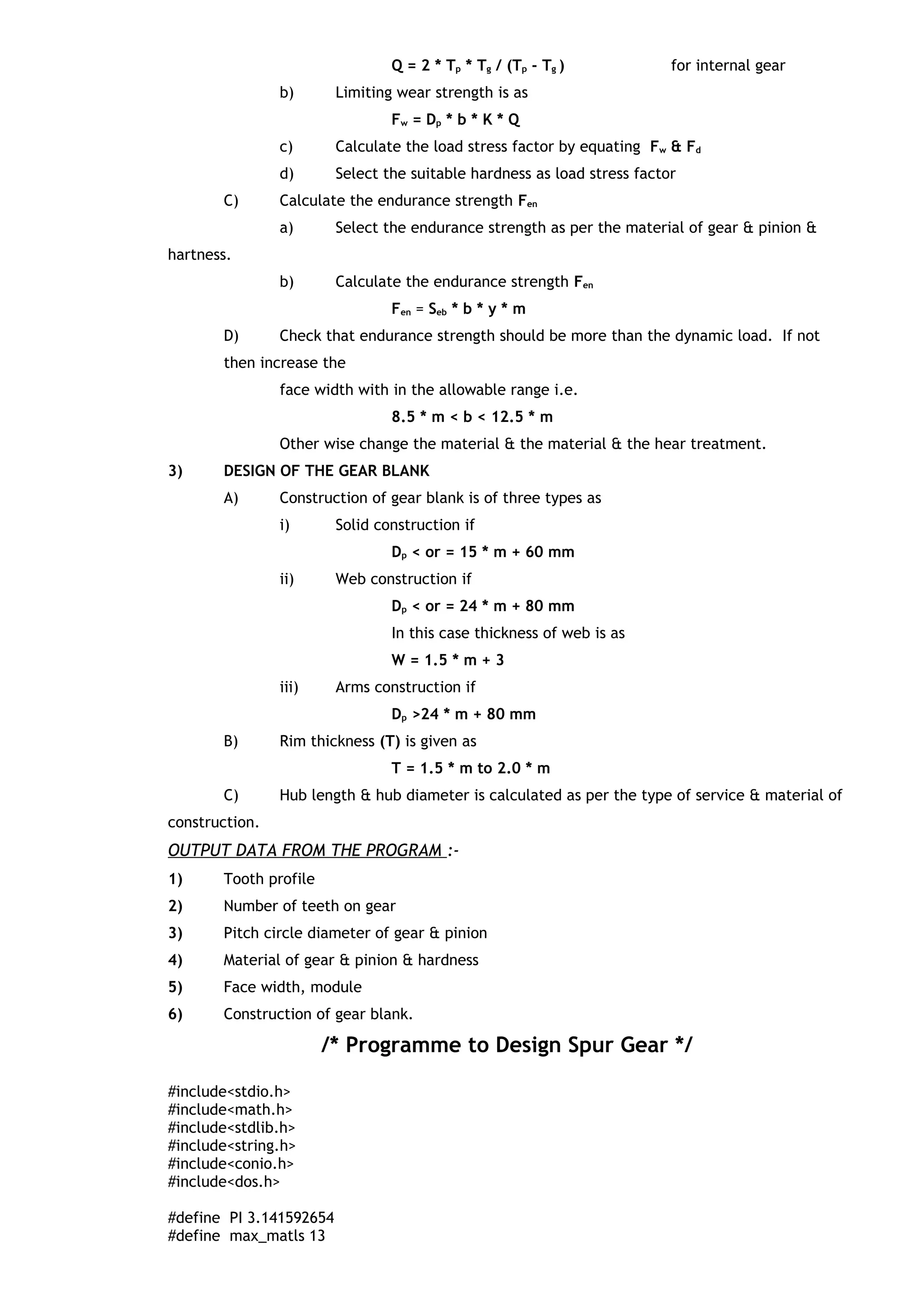

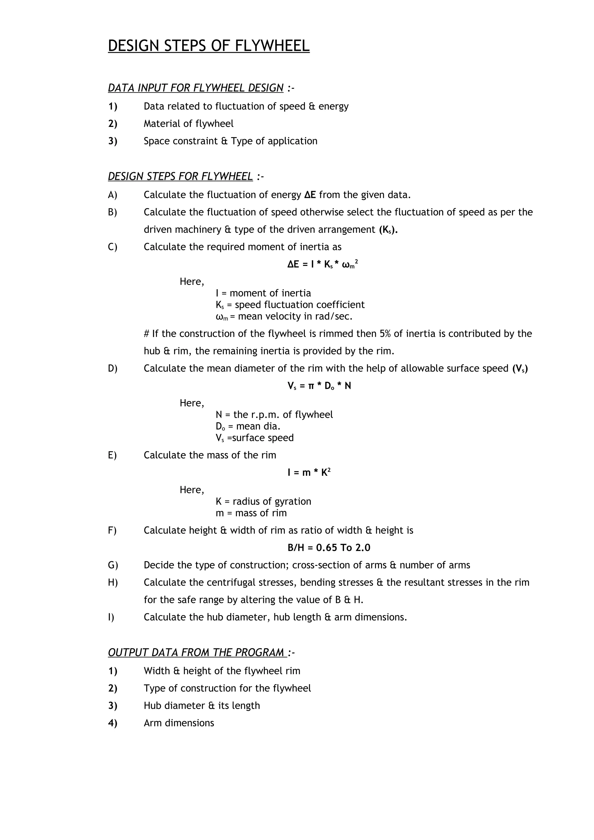
![#include<stdio.h>
#include<conio.h>
#define PI 3.141592654
#define max_matls 5
#define max_input 4
void main()
{
float T,fs,fcb,fsf,fsf1,fsf2,d,D,L,l,w,t,fsk,fck,fsk1,fck1,tf;
float D1,d1,D2,i1,fsb,tp;
int n,j,i;
char matl[max_matls][25],matl_in[max_matls][25],Mtl;
float SS[max_matls]={0},CS[max_matls]={0};
FILE *fp;
clrscr();
fflush(stdin);
clrscr();
printf("nEnter value of torque (Newton-mm) ");
scanf("%f",&T);
/*printf("nEnter value of shear stress for shaft (Newton-mm2) ");
scanf("%f",&fs);
printf("nEnter value of shear stress for flange material (Newton-mm2) ");
scanf("%f",&fsf);*/
if((fp=fopen("CPdata.dat","r"))==NULL)
{
printf("Unable to Openn");
printf("Sorry!!! Please Try Again");
getch();
exit(0);
}
else
{
printf("nFile Opened Successfully!");
printf("nMaterialtShear StresstCrushing Stress");
for(i=0;i<=max_matls-1;i++)
{
fscanf(fp,"%s%f%f",&matl[i],&SS[i],&CS[i]);
printf("n%stt%ft%f",matl[i],SS[i],CS[i]);
}
for(i=0;i<=3;i++)
{
if(i==0)
printf("nEnter Material for Shaft : ");
else
{
if(i==1)
printf("nEnter Material for Flange Coupling](https://image.slidesharecdn.com/camdpractical-150318103014-conversion-gate01/75/Computer-Aided-Manufacturing-Design-86-2048.jpg)

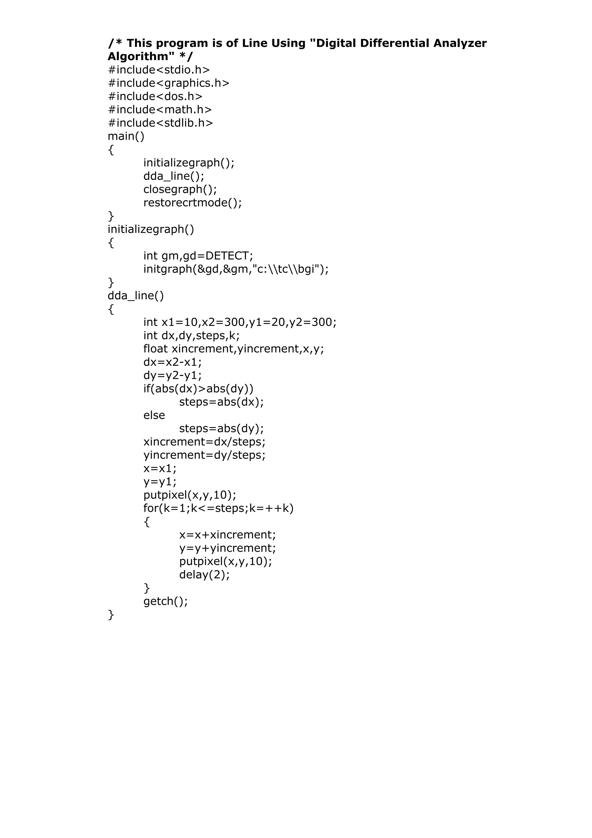
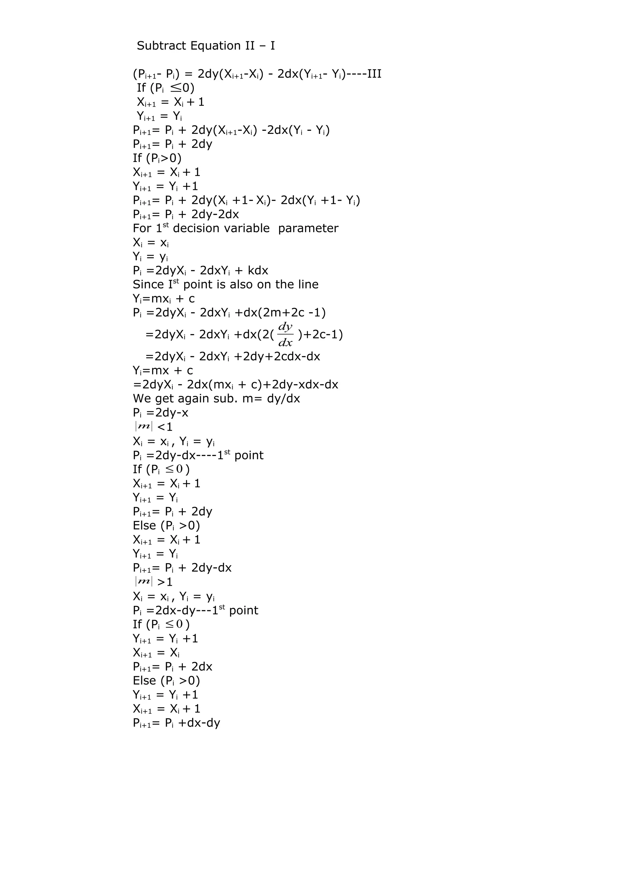
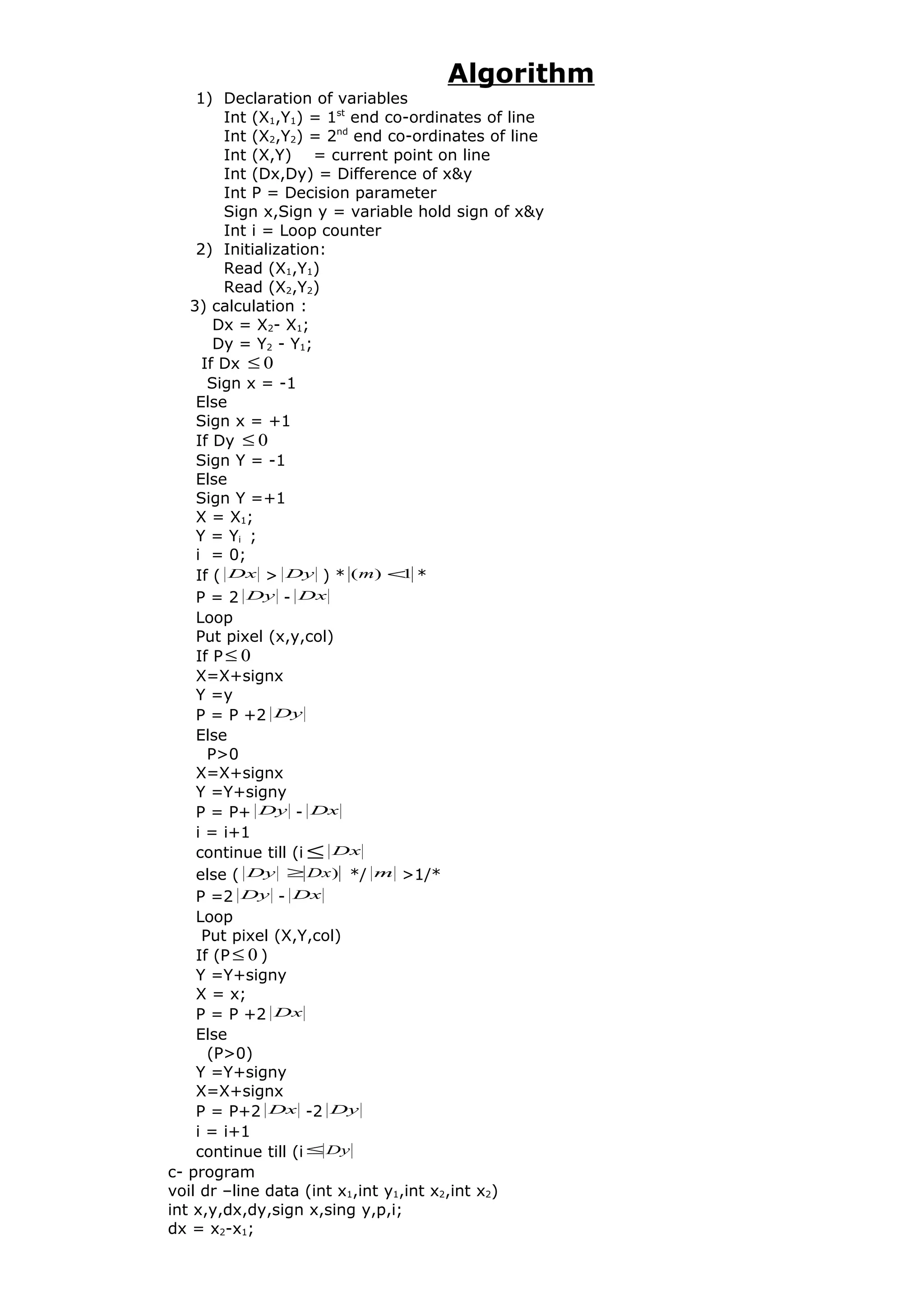
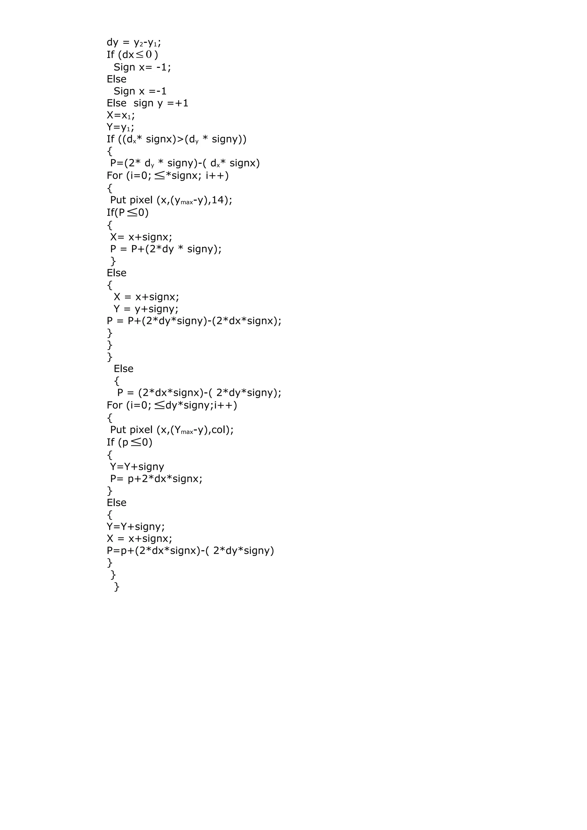
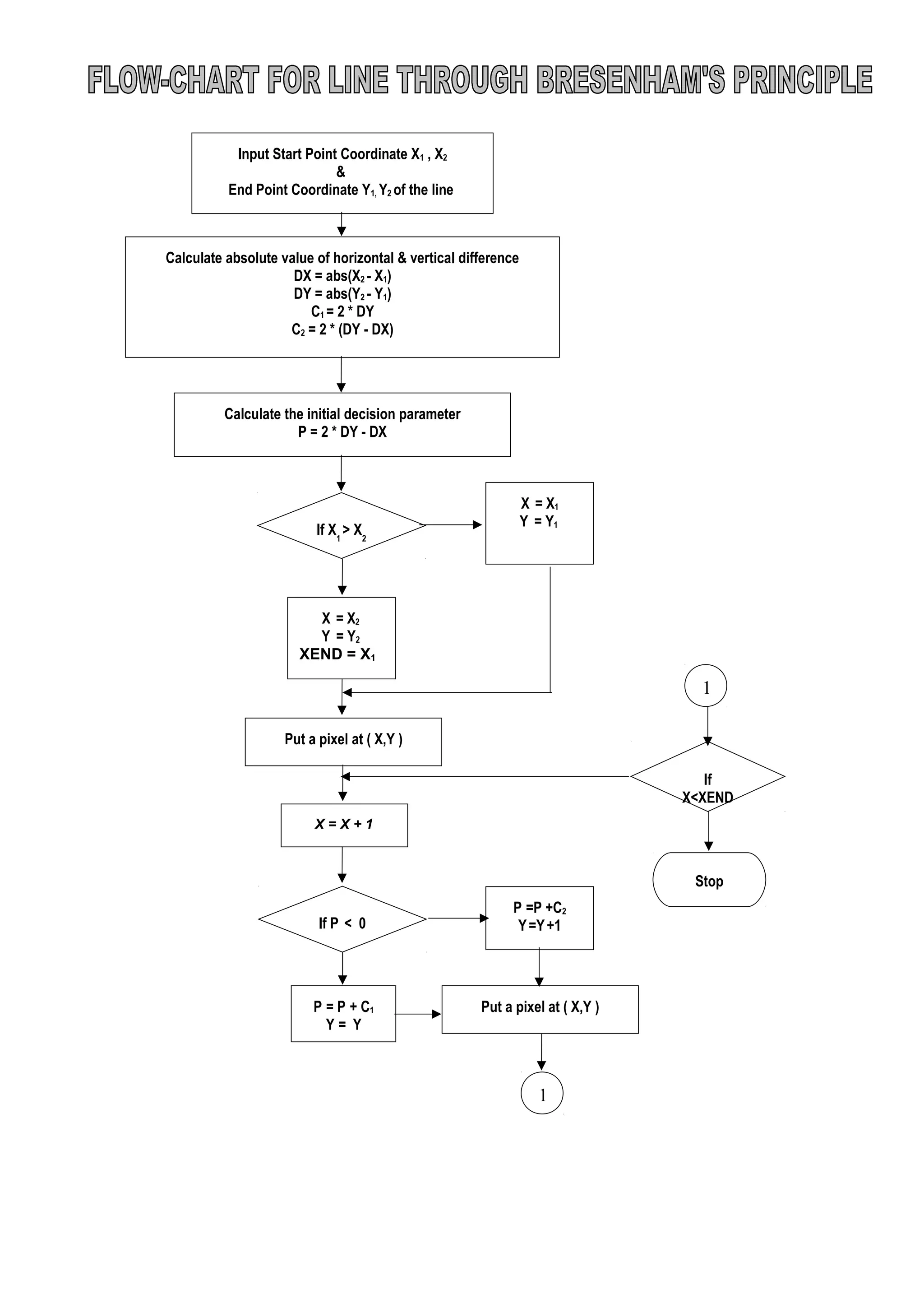
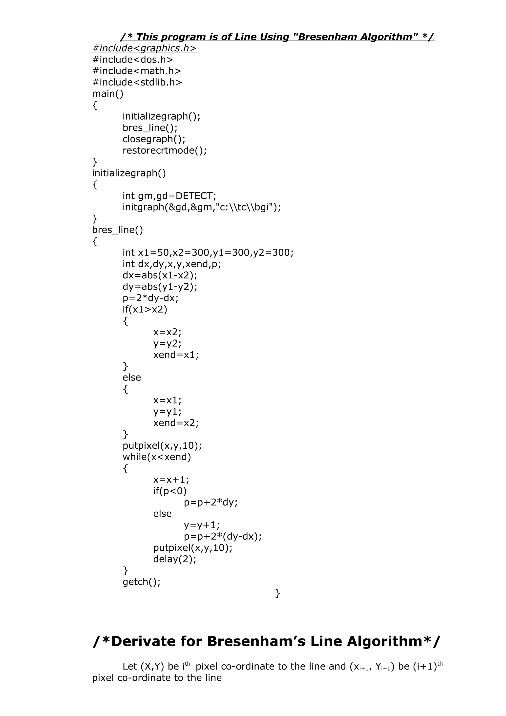
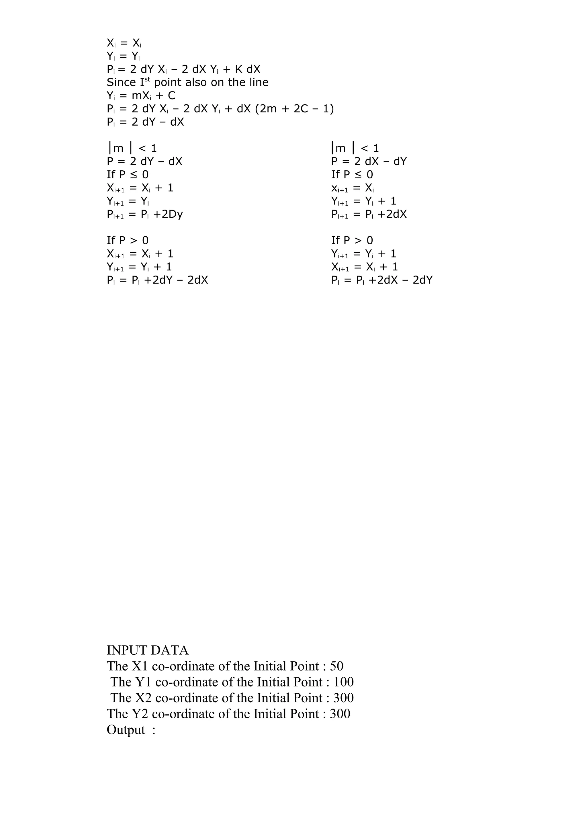
This document describes the Bresenham's line drawing algorithm. It begins with the derivation of the algorithm, showing how it determines which pixel coordinates (xi+1, yi+1) are closest to the line between points (xi, yi) and (xi+1, yi+1) when m < 1. It then provides the algorithm steps, which include calculating differences, initializing variables, and using a decision parameter P to determine whether to increment x or y at each step. Finally, it provides a C program example to draw a line using the Bresenham's algorithm.