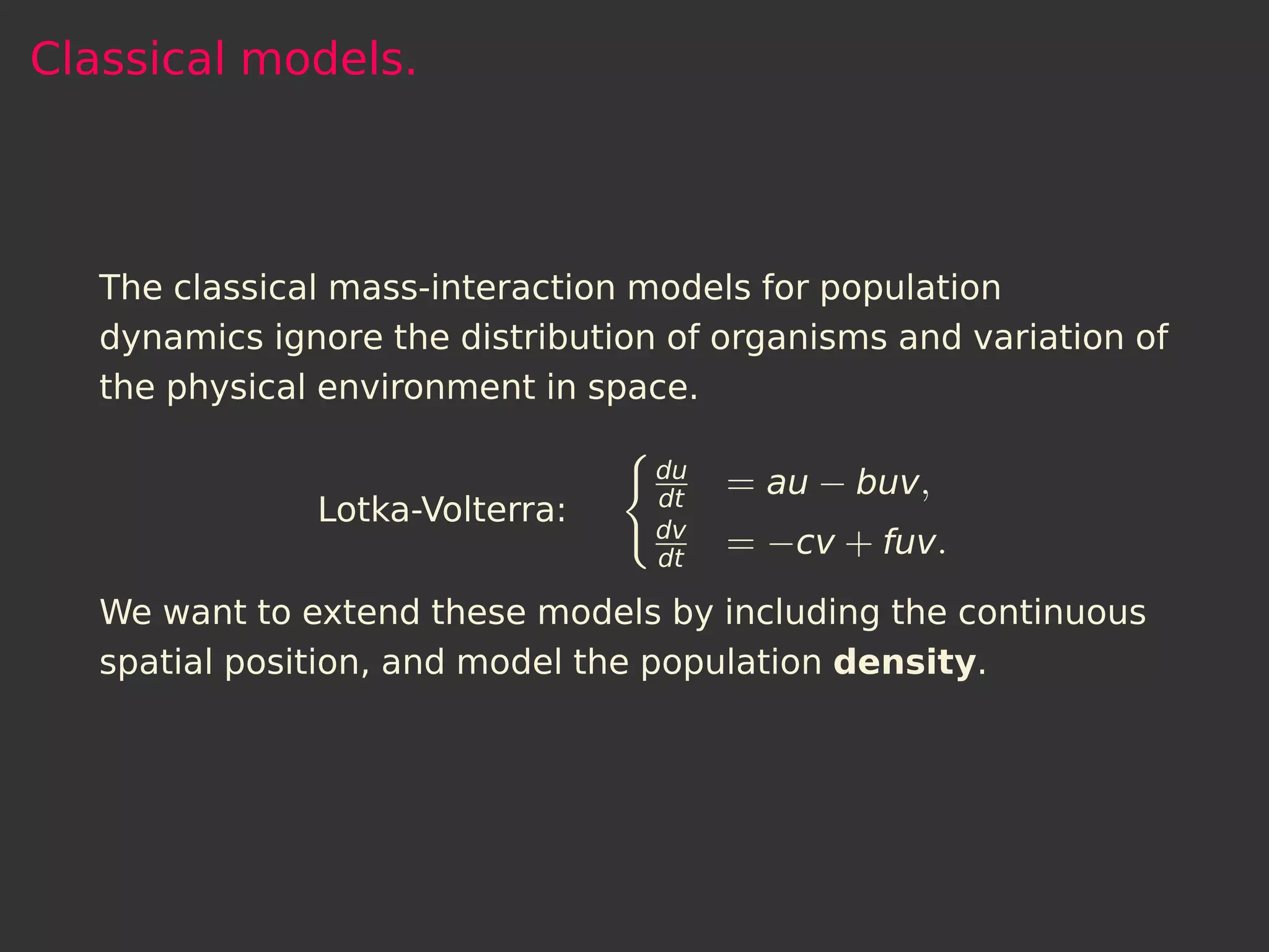
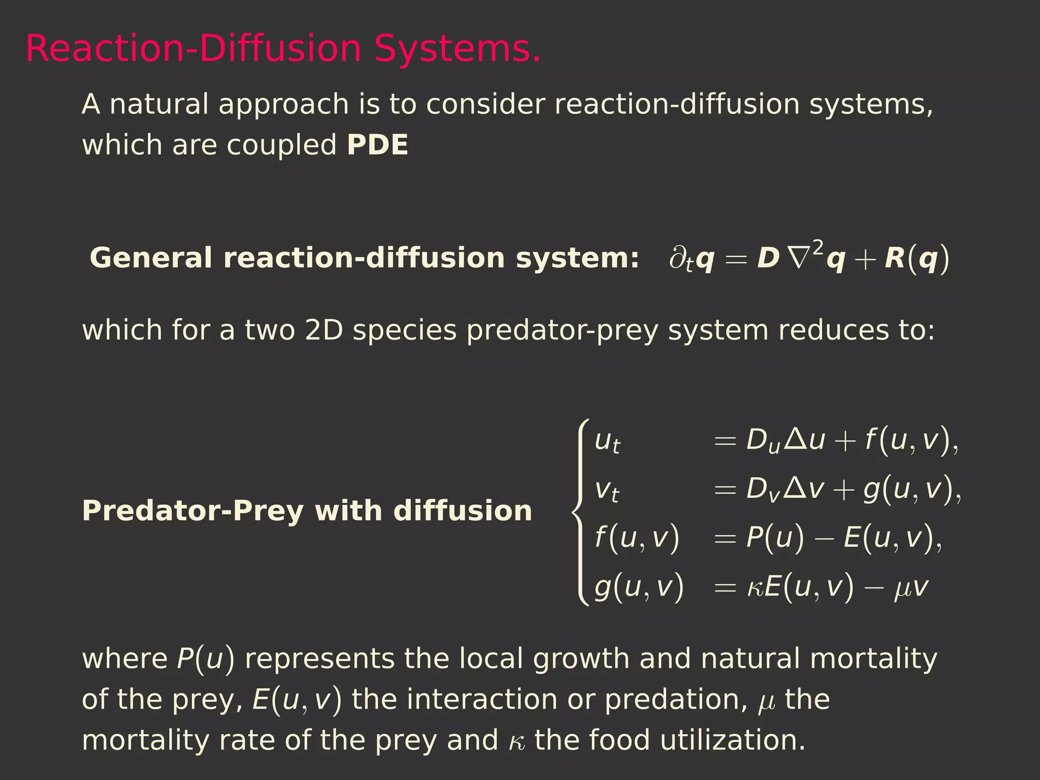
This document summarizes a presentation on numerically solving spatiotemporal models from ecology by implementing an implicit finite difference method in C++. It discusses classical population dynamics models, extending these to include continuous spatial position by using reaction-diffusion systems. It describes discretizing the domain and deriving finite-difference schemes, then solving the equations using GMRES with an ILU preconditioner. Questions addressed include convergence rates and modeling plankton dynamics.

1. Numerical solution of spatiotemporal models
from ecology
Implementing implicit FDM in C++
Kyrre Wahl Kongsgaard
University of Amsterdam
http://student.science.uva.nl/∼kyrre/
Introduction to Computational Science project
presentation – November 1, 2010

2. Classical models.
The classical mass-interaction models for population
dynamics ignore the distribution of organisms and variation of
the physical environment in space.
du
dt
= au − buv,
Lotka-Volterra:
dv
dt
= −cv + fuv.
We want to extend these models by including the continuous
spatial position, and model the population density.

3. Reaction-Diffusion Systems.
A natural approach is to consider reaction-diffusion systems,
which are coupled PDE
2
General reaction-diffusion system: ∂t q = D q + R(q)
which for a two 2D species predator-prey system reduces to:

ut
 = Du ∆u + f (u, v),


v
t = Dv ∆v + g(u, v),
Predator-Prey with diffusion
f (u, v) = P(u) − E(u, v),



g(u, v) = κE(u, v) − µv

where P(u) represents the local growth and natural mortality
of the prey, E(u, v) the interaction or predation, µ the
mortality rate of the prey and κ the food utilization.

4. Dimensionless form and discretization of the domain.
A specific choice for P(u),E(u, v), κ and µ is used to model a
Zooplankton-Phytoplankton aquatic community, here in
dimensionless form.

uv
ut
 = ∆u + u(1 − u) − u+ h
,

= ∆v + k uuvh − mv,

v
t +
Plankton interations:
 u · n = 0, (x, y) ∈ ∂Ω,



v · n = 0, (x, y) ∈ ∂Ω

We discretize space Ω = [a, b]2 by choosing a finite number of
equally spaced points, (xi , yj ) = (i∆x, j∆y), and time by a
countable number of points 0 = t0 , t1 , . . . , where tm = m∆t.

5. Finite-difference scheme.
Inserting the approximations for the time and space
derivatives

um ≈ u(xi , yj , tm ) = u(i∆x, j∆y, m∆t),
 i,j

um+1 −um

 ∂ u(xi ,yj ,tm )
≈ i,j ∆t i,j ,


∂t
2 um+1j −2um+1 +um+,j1
 ∂ u(xi ,yj ,tm ) ≈ i−1, i,j i+1
,
 2 ∂ x2 ∆x 2


 ∂ u(xi ,yj ,tm )
 um+1 −2um+1 +um+1
i,j−1 i,j i,j+1

∂ y2
≈ ∆y 2
into our PDEs we derive a finite-difference equation.
um+1 −um um+1 −2um+1 +um+1 um+1 −2um+1 +um+1
i ,j i,j i−1,j i,j i+1,j i,j−1 i,j i,j+1
= + + f (umj+1 , vimj+1 ),
∆t ∆x2 ∆y 2 i, ,
um+1 vm+1
i ,j i,j
(1 + 4 dt
)umj+1 −2 dt
(um+,j1
+ ui−11 j + umj+1 + ui,j+11 ) = umj + dt(umj+1 (1 − umj+1 ) +
m+ m
i, )
dx2 i, dx2 i+1 , i, +1 − i, i, um+1 +h
i,j

6. Ax = b
If we now number the grid points in ”natural order” we get the
two equations
Aum+1 = um + dtf(um+1 , vm+1 ),
Avm+1 = vm + dtg(um+1 , vm+1 )
in order to avoid updating the matrix at each step we set dt
sufficiently small and work with:
Aum+1 = um + dtf(um , vm ),
Avm+1 = vm + dtg(um , vm )

7. Solving the equations. I
We now need to solve the systems where
2 2
A ∈ R(N+1) ×(N+1) = RM
 
I+H −2I 0 0
 −I I + H −I 
 
 .. .. .. 
A=
 . . . 

 .. .. .. 
 . . . −I 
0 −2I I + H
 
4 −2 0 0
−1 4 −1 
 
dt  .. .. .. 
H= 2
 . . . 
dx 
 .. .. ..


 . . . −1
0 −2 4

8. Solving the equations. II
Dense LU factorize one time O(M3 ) and then iterate over t
solving for u and v. Memory O(M2 ).
Use a special sparse LU factorization/solver for a
3
tridiagonal block matrix. O(M 2 ) flops, O(NlogN) memory.
An iterative method, e.g. Jacobi, GMRES or BiCGSTAB.
Direct computation, A−1 , then solving for u and v
amounts to matrix-vector computation.
Here we decide, mainly due lack of memory, to exploit the
sparse structure of the matrix in combination with GMRES and
the ILU to speed up convergence.

9. The Progam.
/ / read the sparse matrix
CompCol_Mat_double A;
readtxtfile_mat ( " matrix . t x t " , &A ) ;
/ / i n i t i a l conditions
VECTOR_double u , v ;
readtxtfile_vec ( "u_0 . t x t " , &u ) ;
readtxtfile_vec ( "v_0 . t x t " , &v ) ;
MATRIX_double H( r e s t a r t +1, restart , 0 . 0 ) ;
CompCol_ILUPreconditioner_double M(A ) ; / / ILU precond .
output (u, 0 , p r e y _ f i l e ) ; output ( v , 0 , p r e d _ f i l e ) ;
f o r ( t = dt ; t <= t_end && ( ! result_1 && ! result_2 ) ; t += dt ) {
F (b1 , u , v , dt ) ; G(b2 , u , v , dt ) ; / / reaction terms + . . .
set_gmres_parameters ( maxit , restart , t o l ) ; /
result_1 = GMRES(A, u , b1 , M, H, restart , maxit , t o l ) ;
set_gmres_parameters ( maxit , restart , t o l ) ;
result_2 = GMRES(A, v , b2 , M, H, restart , maxit , t o l ) ;
output (u , t , p r e y _ f i l e ) ; output ( v , t , p r e d _ f i l e ) ;
}

10. Questions?

11. Holling Type II Functional Response.
The predator spends it time doing on two things.
Searching for prey
Prey handling which includes: chasing, killing, eating and
digesting.
Holling Type II: ”Search rate is constant. Plateau represents
predator saturation. Prey mortality declines with prey density.
Predators of this type cause maximum mortality at low prey
density. For example, small mammals destroy most of gypsy
moth pupae in sparse populations of gypsy moth. However in
high-density defoliating populations, small mammals kill a
negligible proportion of pupae.”
-
http://home.comcast.net/ sharov/PopEcol/lec10/funcresp.htm

12. ”How good is our approximation actually? What
about the rate-of-convergence?”
Since we cannot solve the problem analytically we must use a
fine approximate solution (i.e. small ∆t and ∆x2 ) - Ui, jm to
estimate the rate of convergence.
E(∆x, ∆y, ∆t )m = max|um − Um |
i,j i,j
E(∆x,∆y,∆tsmall )m
Now we compute R∆x,∆y = ∆x ∆x and
E( 2
, 2
,∆tsmall )
E(∆xsmall ,∆ysmall ,∆t m )
R ∆t =
E(∆xsmall ,∆ysmall , ∆t )
2
Assuming that E ≈ c∆xα , we estimate α by computing
logR∆x,∆y
α ≈ log∆x1 /∆x2 .
I have not done this, but plausible reasoning leads me to
believe the error is O(∆x2 + ∆t ). (for ∆x = ∆y)

13. Plankton Dynamics. Motivation.
Plankton are floating organisms of many different phyla
living in the pelagic of the sea.
Together, phyto- and zooplankton form the basis for all
food chains and webs in the sea.
The abundance of the plankton species is affected by a
number of environmental factors.
Oxygen and carbondioxide, and other substances are
recycled by phytoplankton,
They are to a large extent subject to water movements.
The question investigated by Medvinsky et al. is: Can
biological factors, such as predator-prey growth and
interactions, be a cause of plankton pattern formation
without any hydrodynamic forcing?