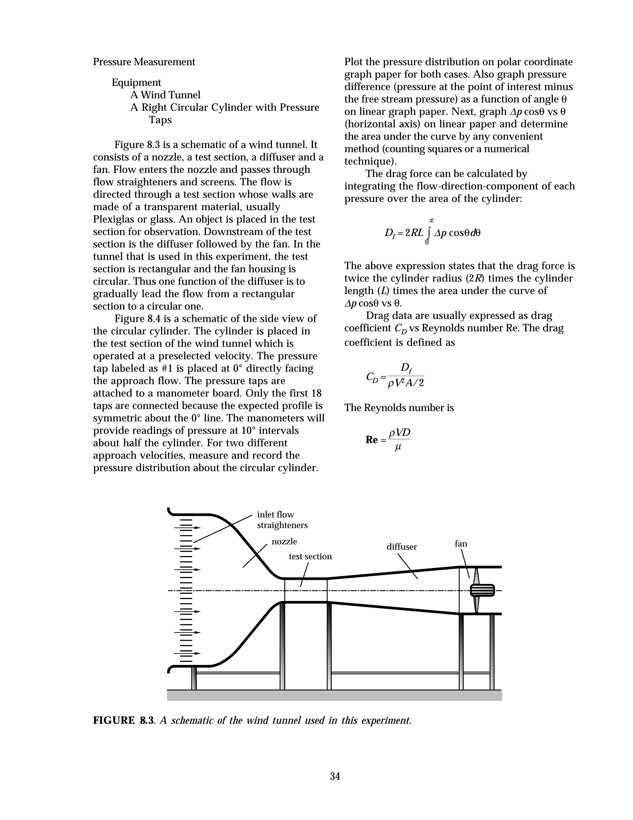
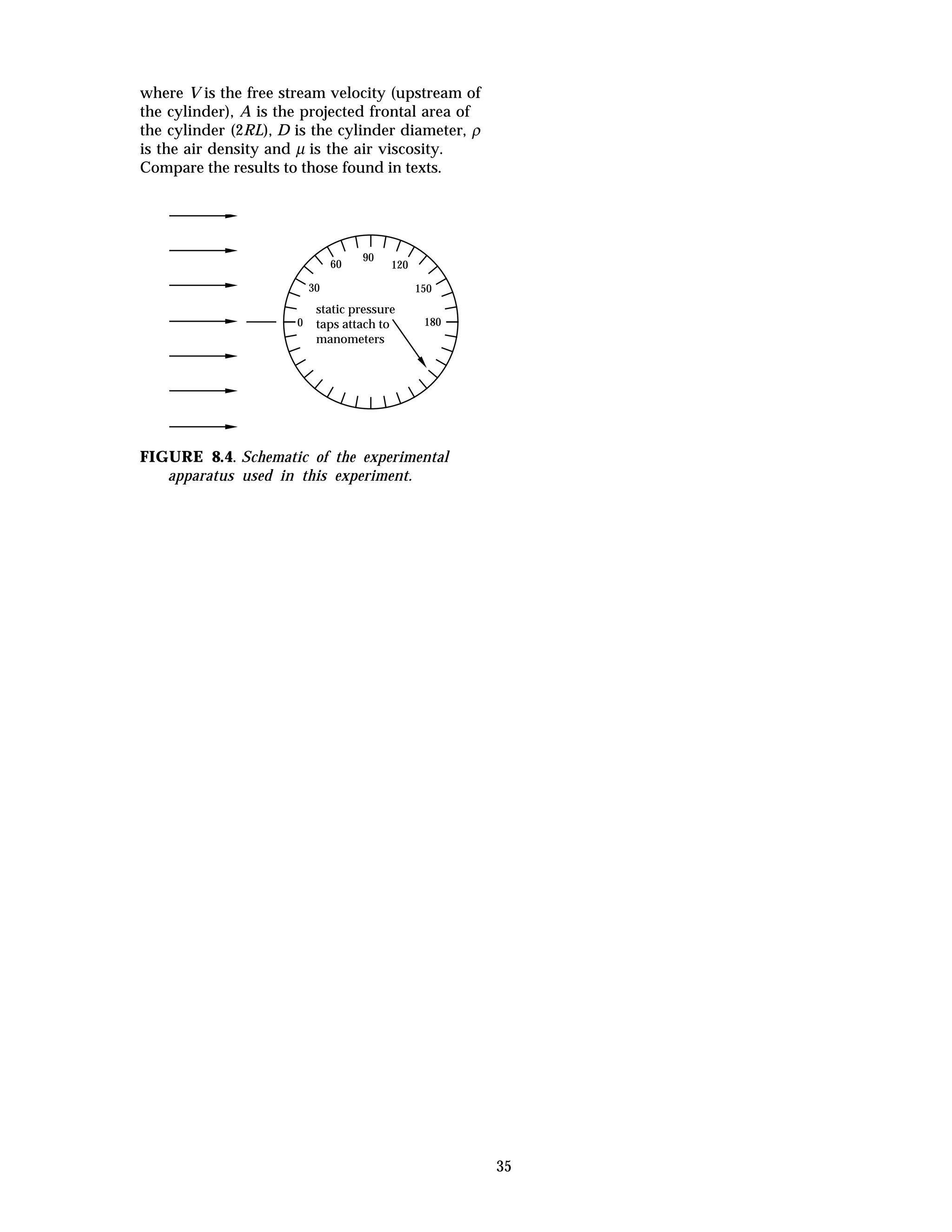
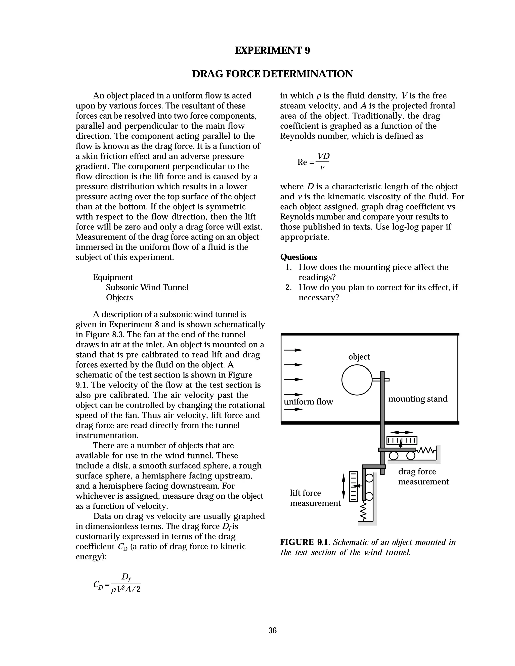
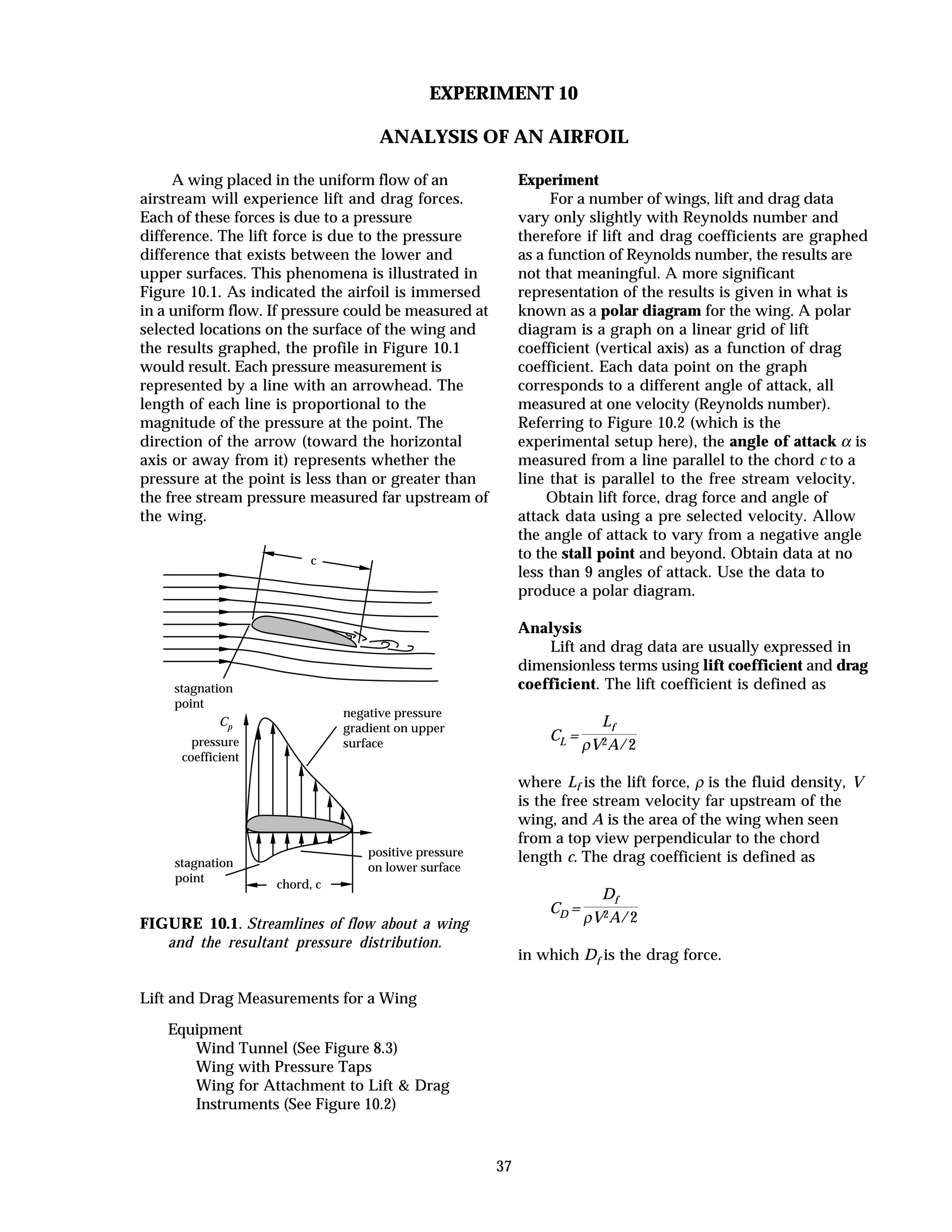
Downloaded 526 times

![48
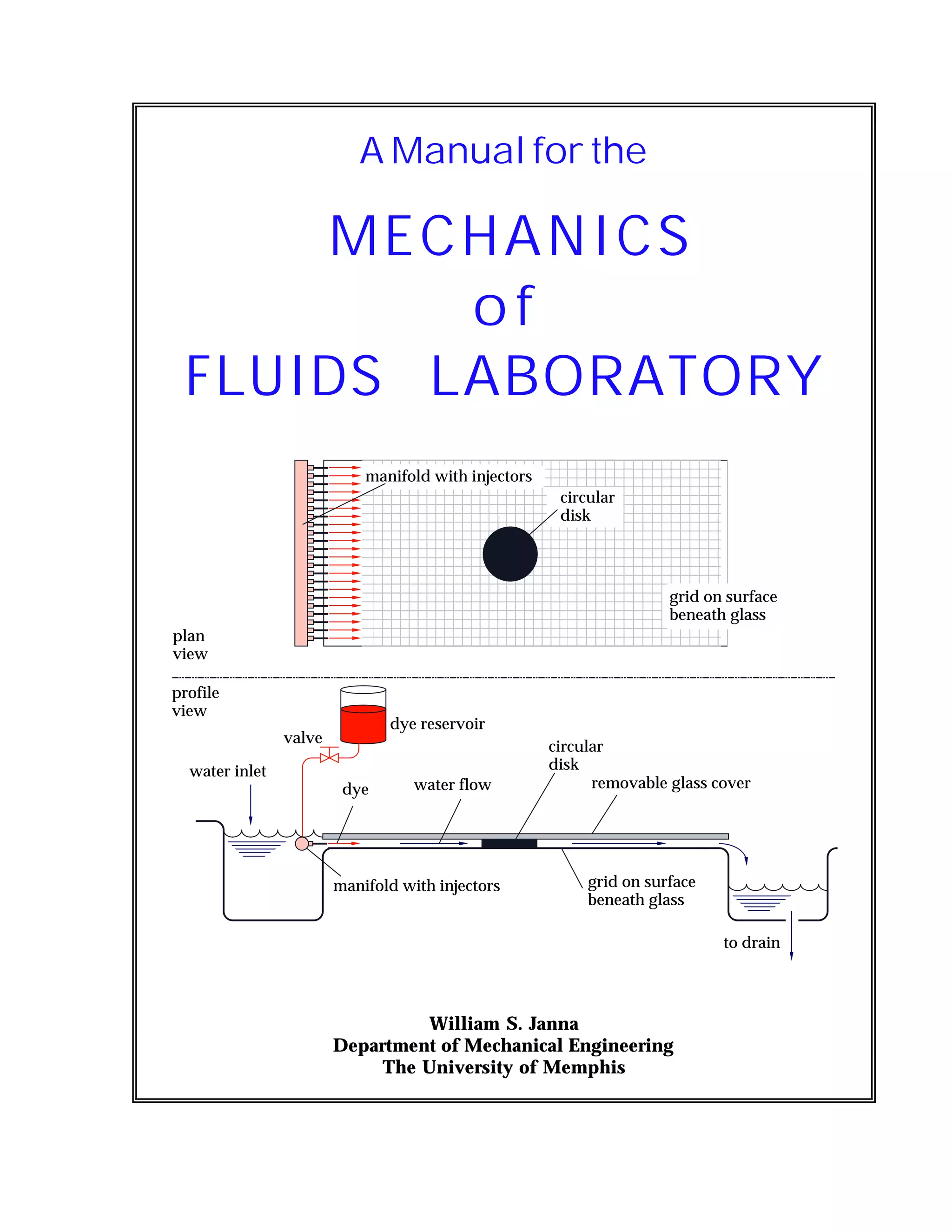
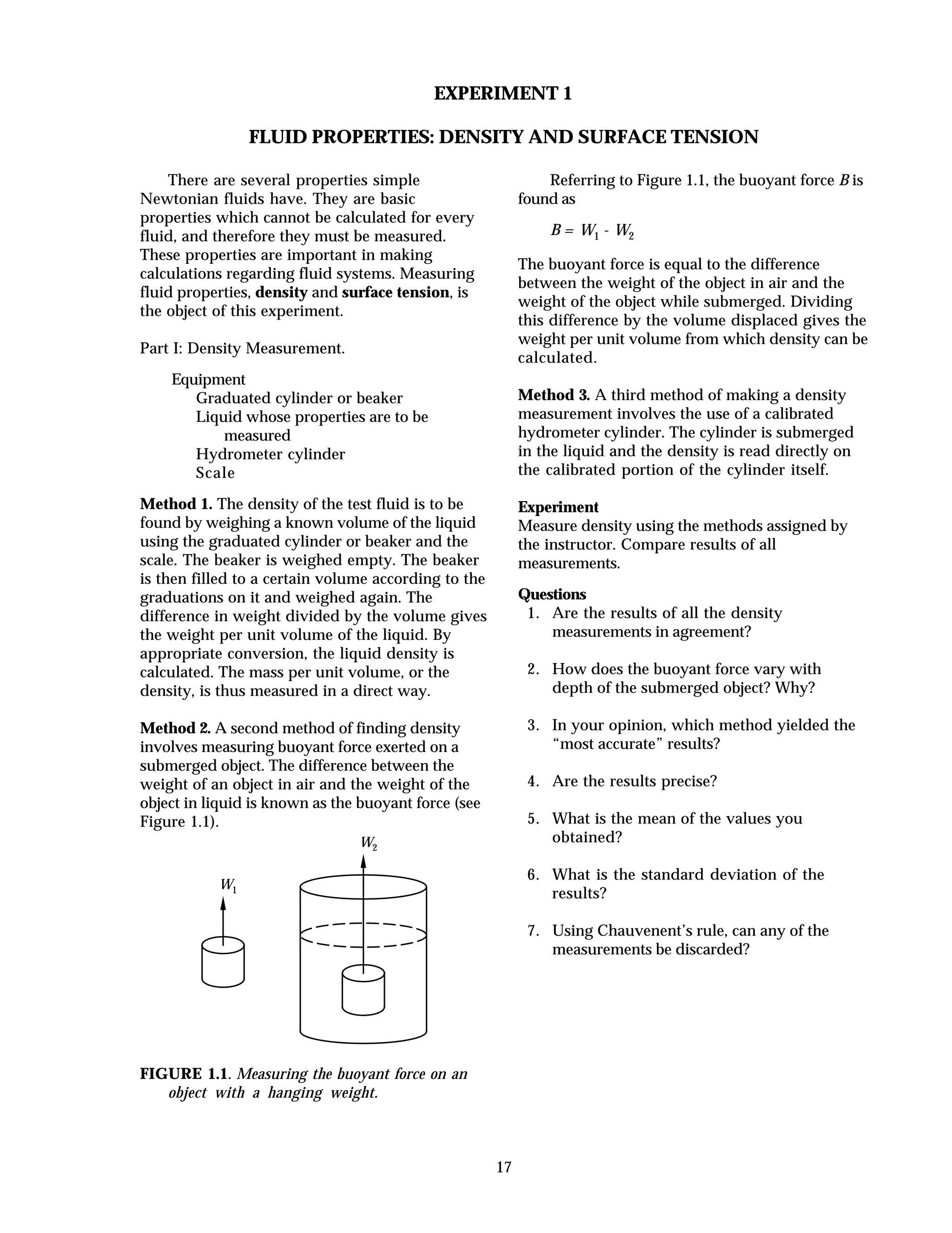
Specific Speed
A dimensionless group known as specific
speed can also be derived. Specific speed is found
by combining head coefficient and flow
coefficient in order to eliminate characteristic
length D:
ωss =
Q
ωD3
1/2
ω2D2
g∆H
3/4
or ωss =
ωQ1/2
(g∆H)3/4 [dimensionless]
Exponents other than 1/2 and 3/4 could be used (to
eliminate D), but 1/2 and 3/4 are customarily
selected for modeling pumps. Another definition
for specific speed is given by
ωs =
ωQ1/2
∆H3/4
rpm =
rpm(gpm)1/2
ft3/4
in which the rotational speed ω is expressed in
rpm, volume flow rate Q is in gpm, total head ∆H
is in ft of liquid, and specific speed ωs is
arbitrarily assigned the unit of rpm. The equation
for specific speed ωss is dimensionless whereas
ωs is not.
The specific speed of a pump can be
calculated at any operating point, but
customarily specific speed for a pump is
determined only at its maximum efficiency. For
the pump of this experiment, calculate its
specific speed using both equations.](https://image.slidesharecdn.com/fluidslabmanual2-140524214604-phpapp01/75/Fluids-lab-manual_2-48-2048.jpg)
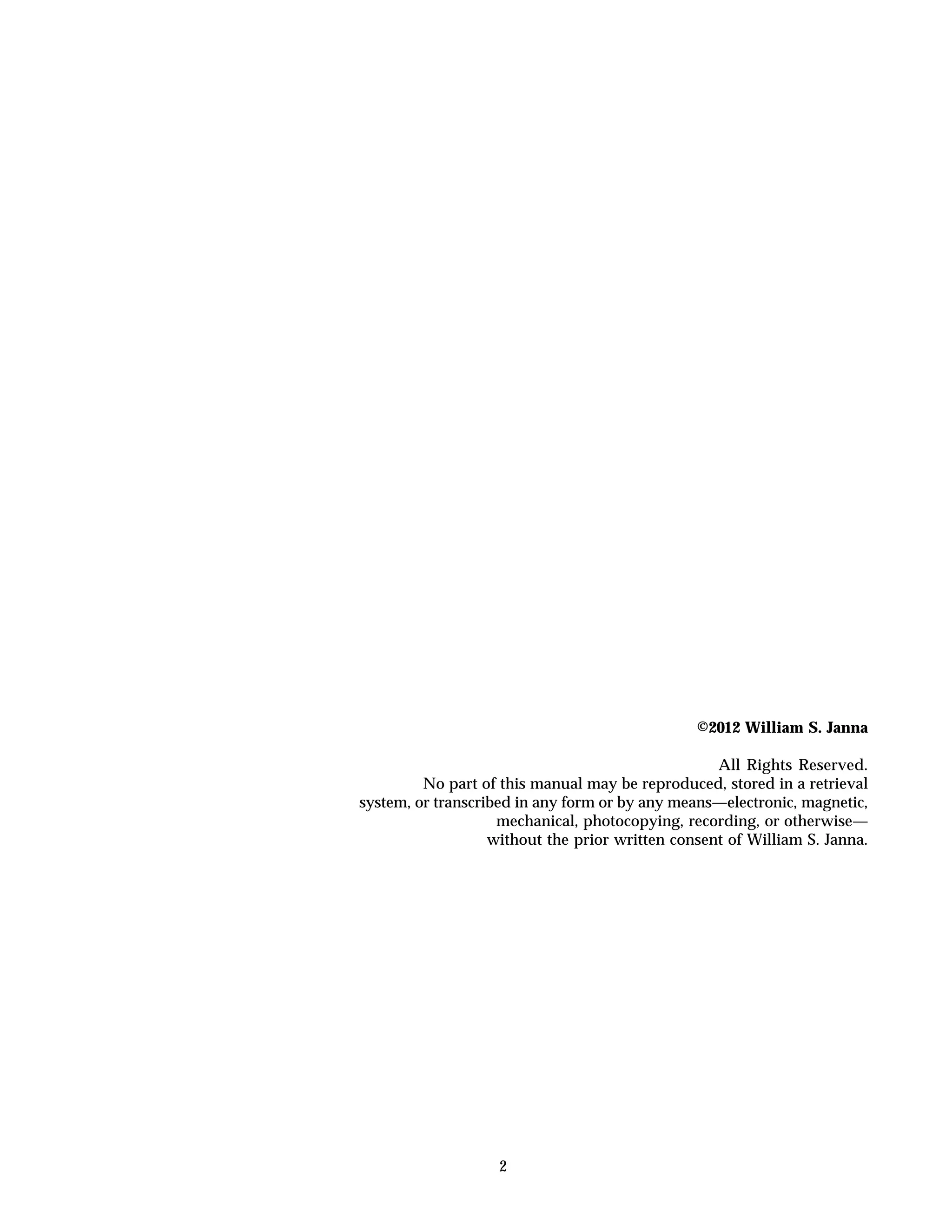
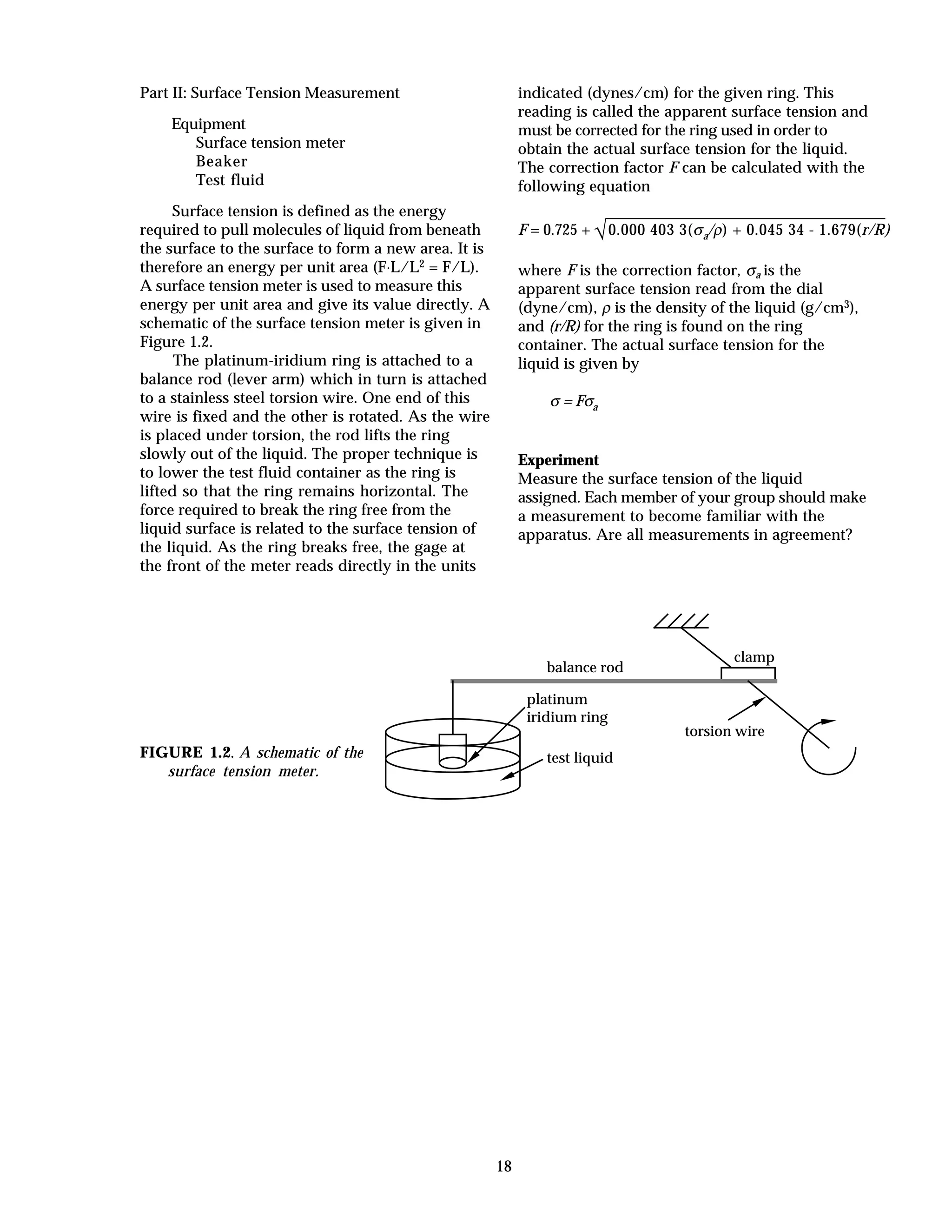
![53
TABLE 15.1. Summary of equations for compressible flow through a venturi or an orifice meter.
·
ms = A2
2p1ρ1 (p2/p1)2/γ [γ/(γ - 1)] [1 - (p2/p1)(γ - 1)/γ
]
1 - (p2/p1)2/γ (D2
4/D1
4)
1/2
(15.1)
·
mac = Cv A2
2p1ρ1 (p2/p1)2/γ [γ/(γ - 1)] [1 - (p2/p1)(γ - 1)/γ
]
1 - (p2/p1)2/γ (D2
4/D1
4)
1/2
(15.2)
Y =
√γ
γ - 1
[(p2/p1)2/γ - (p2/p1)(γ + 1)/γ](1 - D2
4/D1
4)
[1 - (D2
4/D1
4)(p2/p1)2/γ](1 - p2/p1)
(venturi meter) (15.3)
Y = 1 - (0.41 + 0.35β 4)
(1 - p2/p1)
γ
(orifice meter) (15.4)
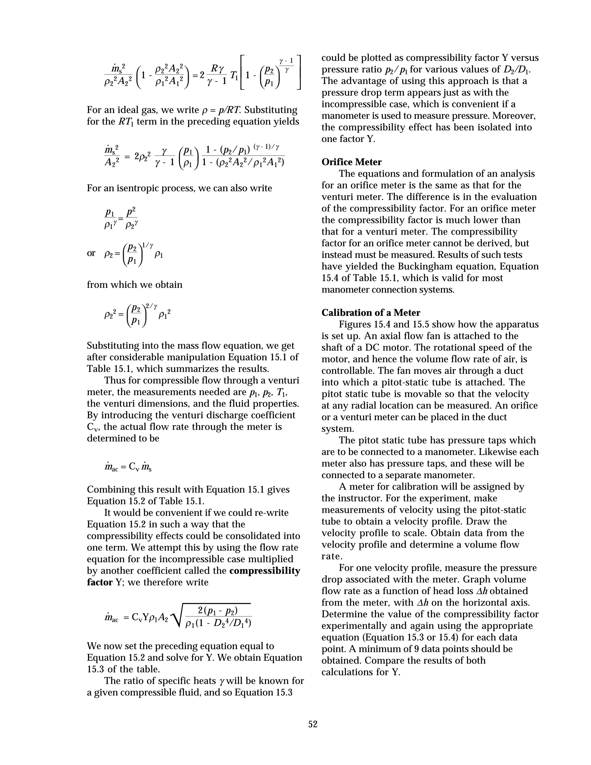
rounded
inlet
outlet ductaxial flow
fan
motor
manometer
connections
pitot-static
tube
venturi meter
FIGURE 15.4. Experimental setup for calibrating a venturi meter.
rounded
inlet
outlet ductaxial flow
fan
motor
orifice plate
manometer
connections
pitot-static
tube
FIGURE 15.5. Experimental setup for calibrating an orifice meter.](https://image.slidesharecdn.com/fluidslabmanual2-140524214604-phpapp01/75/Fluids-lab-manual_2-53-2048.jpg)
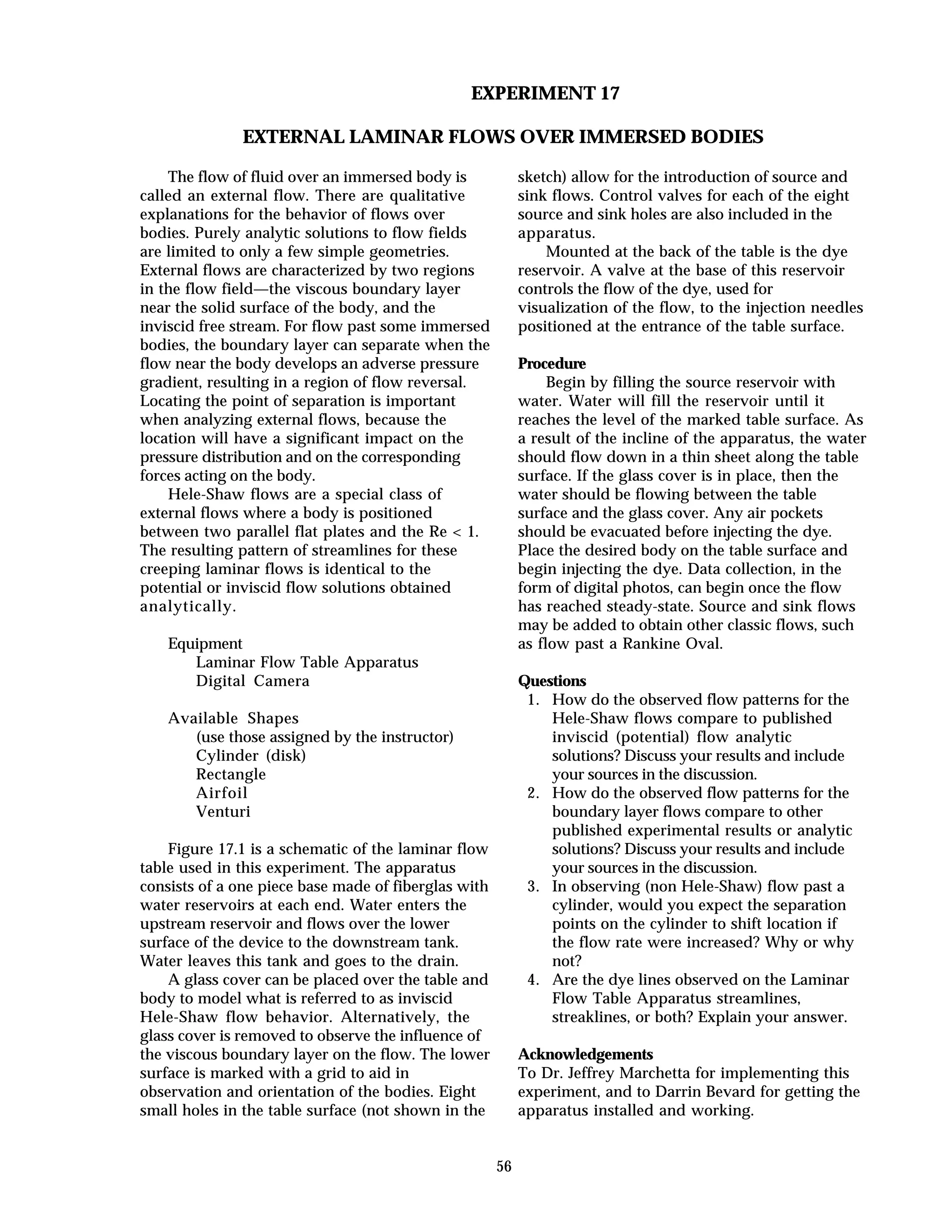
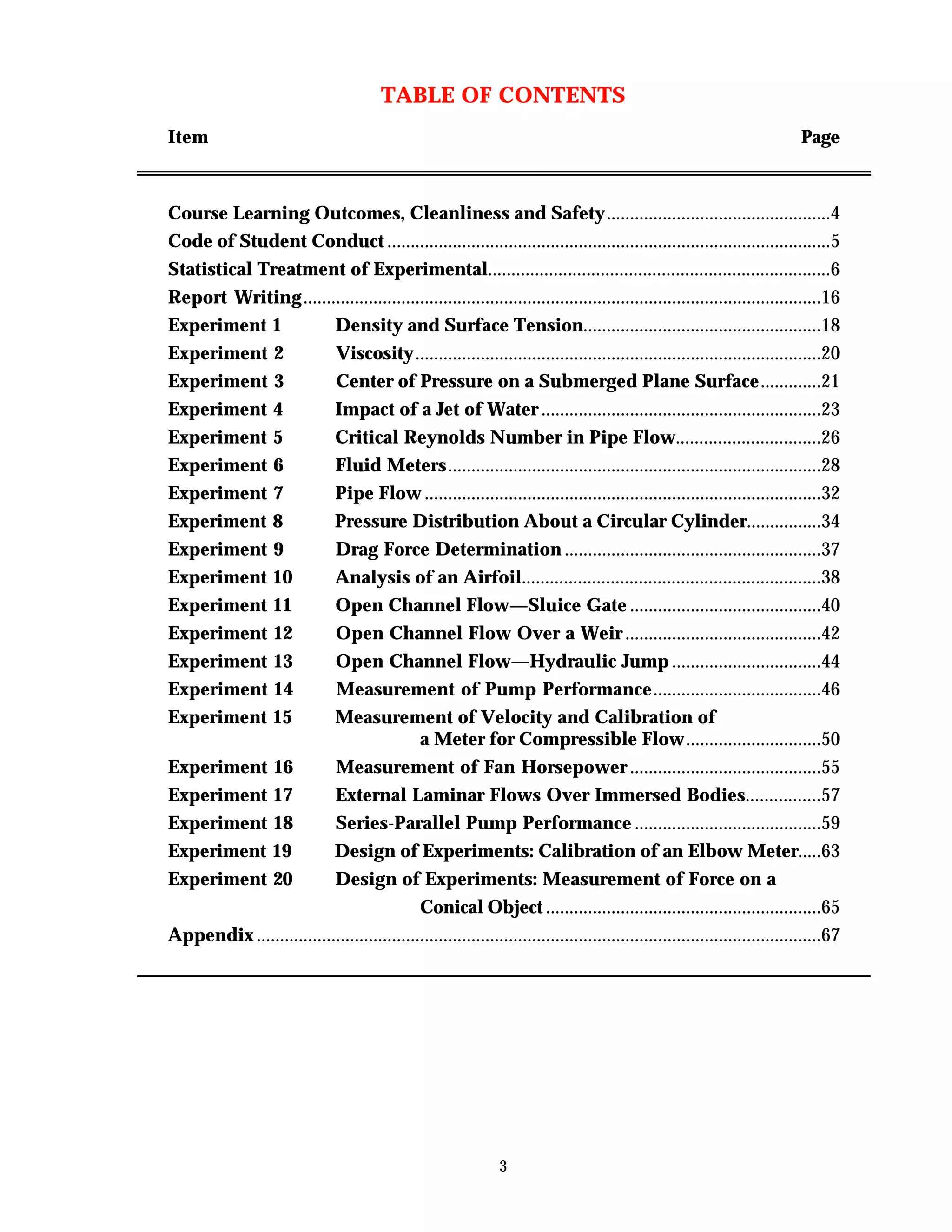
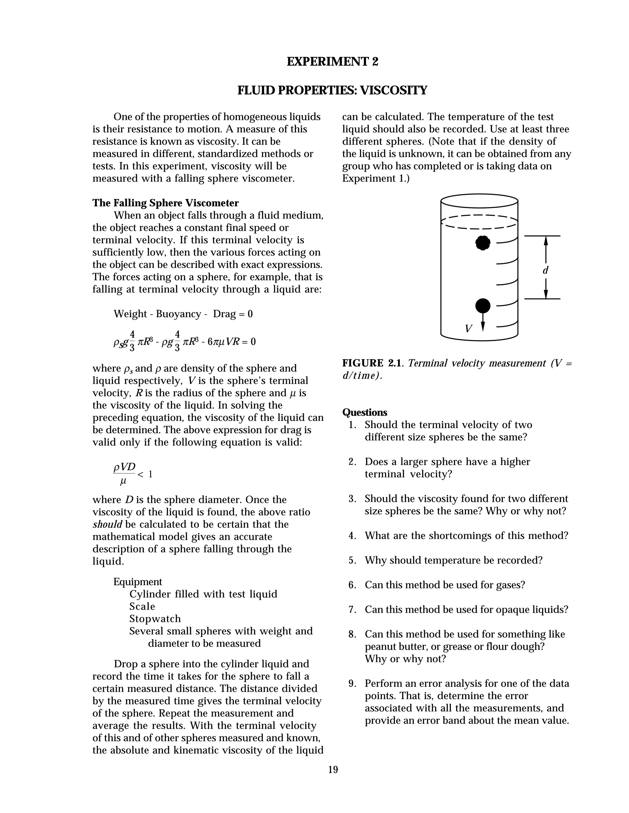
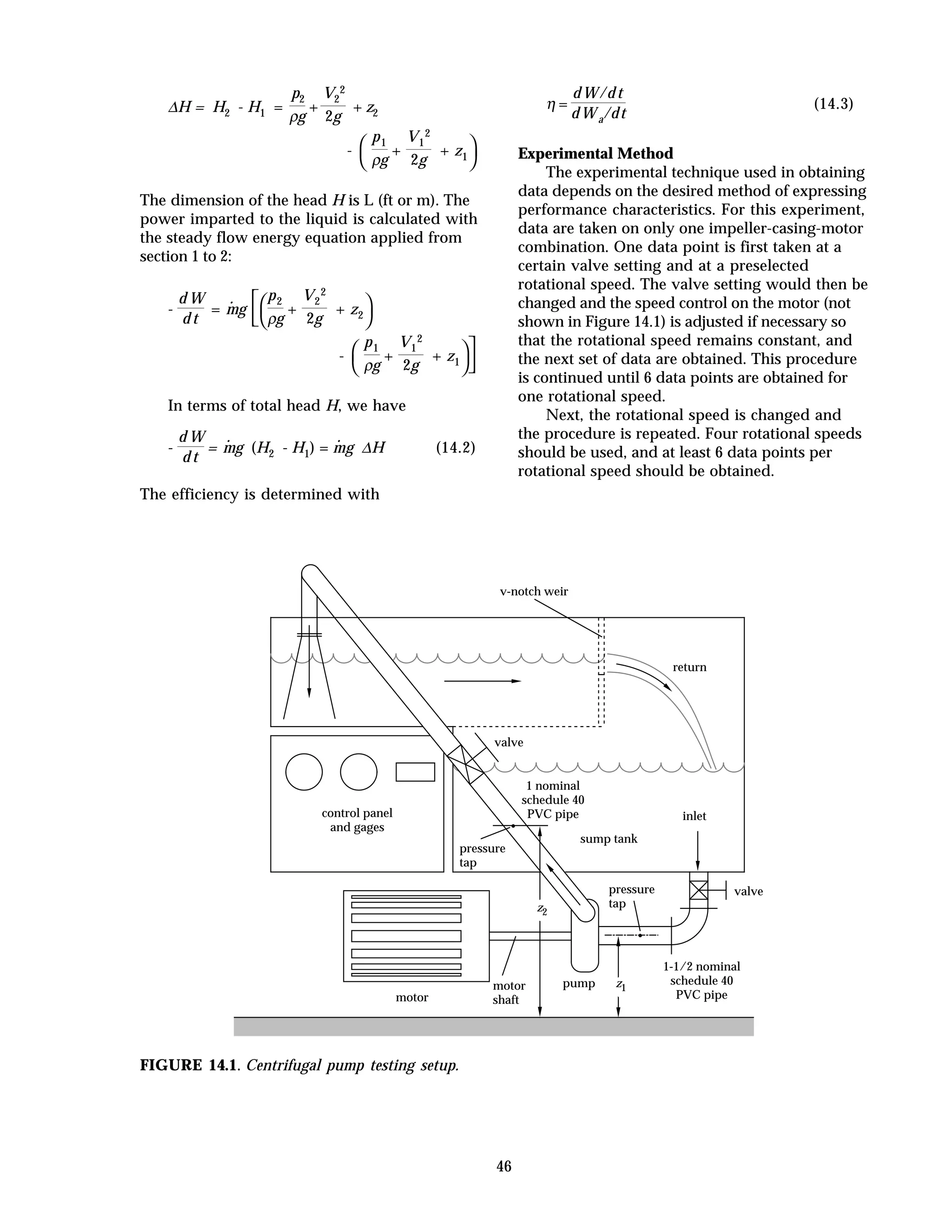
![59
Single Pump Performance
The objective here is to obtain a head flow
curve (∆H vs Q) for a centrifugal pump
operating at one speed.
Procedure
• Launch the program FM21SNGL on the
computer.
• Use pump (1) and be sure that the valves
are set appropriately: valves A, B, and E
are open. Valves C and D are closed.
• Start pump (1); pump (2) should remain off.
Decide on a power setting for pump (1) [such
as 50% or 75% or 100%] and set its controller
accordingly. This setting is used for this
and the subsequent experiments.
• Select “Diagrm” and note the value of the
volume flow rate displayed by the
computer.
• Decide on suitable increments to use for flow
rate so that typically 15 data points are
obtained between zero and maximum flow
rate.
• Close valve E for the condition of no flow
(Q = 0). When the readings on the screen
become sufficiently steady, select “Take
Sample.” This is the first data point. DO
NOT allow the pump to operate at zero
flow for any longer than necessary.
• Open valve E slightly to the first increment
in flow rate decided upon earlier. When
the readings are sufficiently steady, select
“Take Sample.”
• Repeat the previous step for other settings
of valve E, corresponding to increasing
values of flow rate. The last sample point
corresponds to valve E being fully open.
• The recorded data set can now be examined
via any of the selectable options:
“Graphs,” “Tables,” or downloaded into a
spreadsheet. Select the “Graphs” option
and obtain a head versus flow rate curve.
(See software help screens if necessary.)
Series Pump Performance
The objective here is to obtain a head flow
curve (∆H vs Q) for a two identical centrifugal
pumps operating at the same speed, and
operated such the flow leaving pump (1) enters
that of pump (2). When two pumps operate in
series, the combined head versus flow rate
curves is found by adding the heads of the
single pump curves at the same flow rates.
Procedure
• Launch the program FM21SERS on the
computer.
• Use both pumps and be sure that the valves
are set appropriately: valve A is closed.
All other valves are open.
• Start both pumps, and set them on the same
power setting that was used in the single
pump experiment. This setting is used for
this and the subsequent experiment.
• Select “Diagrm” and note the value of the
volume flow rate displayed by the
computer.
• Decide on suitable increments to use for flow
rate so that typically 15 data points are
obtained between zero and maximum flow
rate.
• Close valve E for the condition of no flow
(Q = 0). When the readings on the screen
become sufficiently steady, select “Take
Sample.” This is the first data point. DO
NOT allow the pump to operate at zero
flow for any longer than necessary.
• Open valve E slightly to the first increment
in flow rate decided upon earlier. When
the readings are sufficiently steady, select
“Take Sample.”
• Repeat the previous step for other settings
of valve E, corresponding to increasing
values of flow rate. The last sample point
corresponds to valve E being fully open.
• The recorded data set can now be examined
via any of the selectable options:
“Graphs,” “Tables,” or downloaded into a
spreadsheet. Select the “Graphs” option
and obtain a head versus flow rate curve.
(See software help screens if necessary.)
Parallel Pump Performance
The objective here is to obtain a head flow
curve (∆H vs Q) for a two identical centrifugal
pumps operating at the same speed, and
operated in parallel. Both pumps take in water
from the tank, and discharge the water into a
common line containing the valve at E. When
two pumps operate in parallel, the combined
head versus flow rate curves is found by adding
the flow rates of the single pump curves at the
same head.
Procedure
• Launch the program FM21PARA on the
computer.
• Use both pumps and be sure that the valves
are set appropriately: valve D is closed.
All other valves are open. .
• Start both pumps, and set them on the same
power setting that was used in the single
pump experiment.](https://image.slidesharecdn.com/fluidslabmanual2-140524214604-phpapp01/75/Fluids-lab-manual_2-59-2048.jpg)

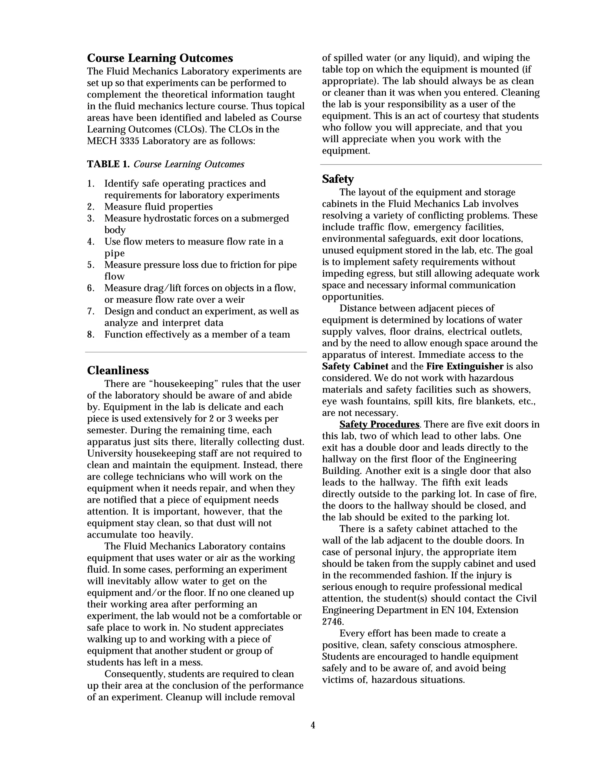
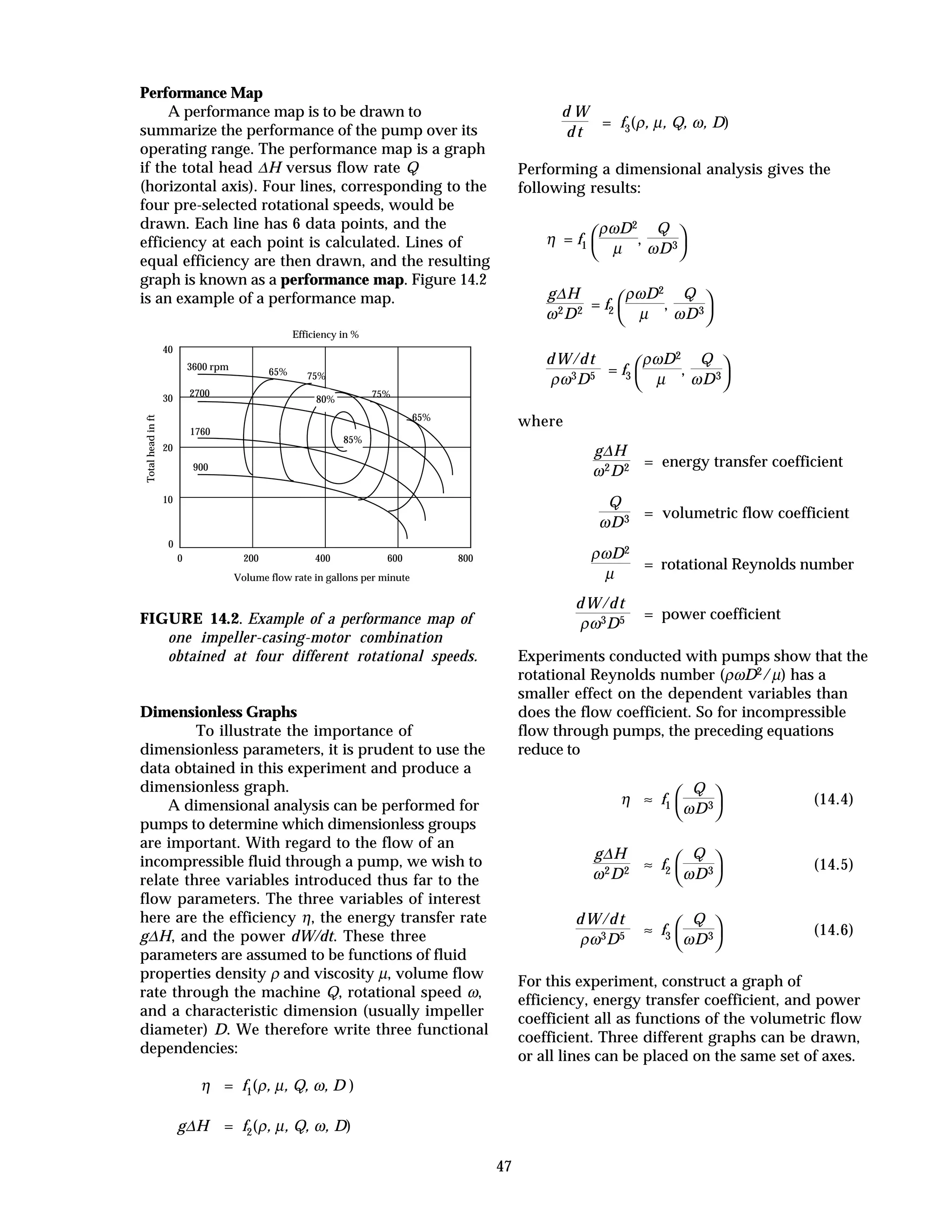
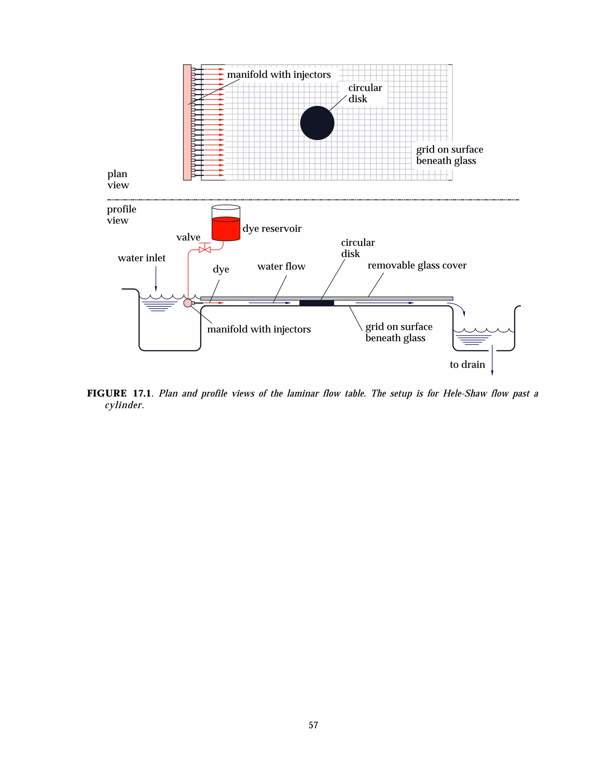
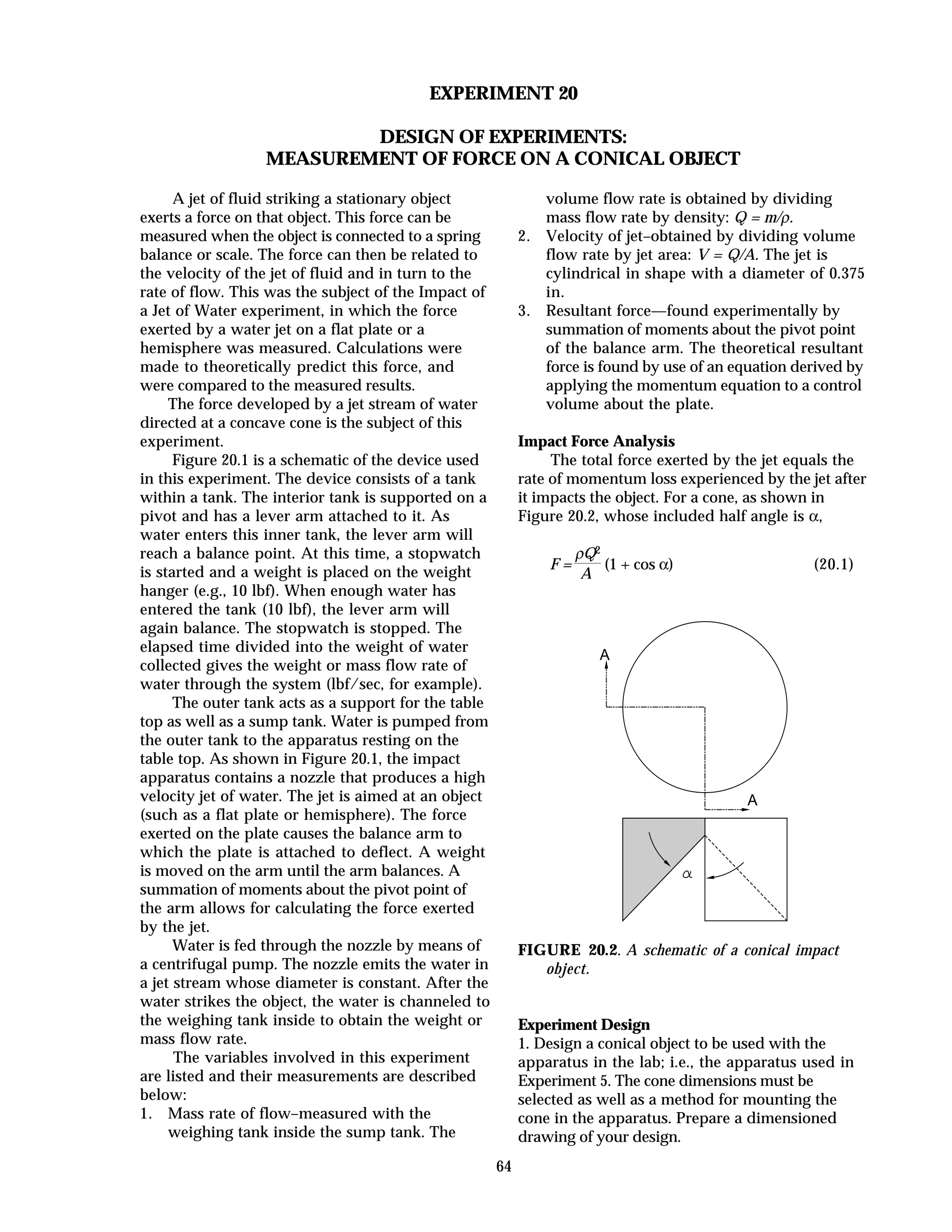
![62
EXPERIMENT 19
DESIGN OF EXPERIMENTS:
CALIBRATION OF AN ELBOW METER
There are many types of meters that can be
installed in a pipeline—venturi, orifice,
rotameter, and turbine-type. These meters can all
be calibrated to provide a reading of the volume
flow rate of fluid through the pipe.
An alternative, less expensive flow meter—
known as an elbow meter—can also be used. For an
existing pipeline containing elbows, an elbow
meter is perhaps the easiest meter to set up. All
that would be required is to drill and tap a couple
of holes in the elbow, and attach them to a
device for measuring pressure drop. Information
on an elbow meter is available from [1]. A sketch
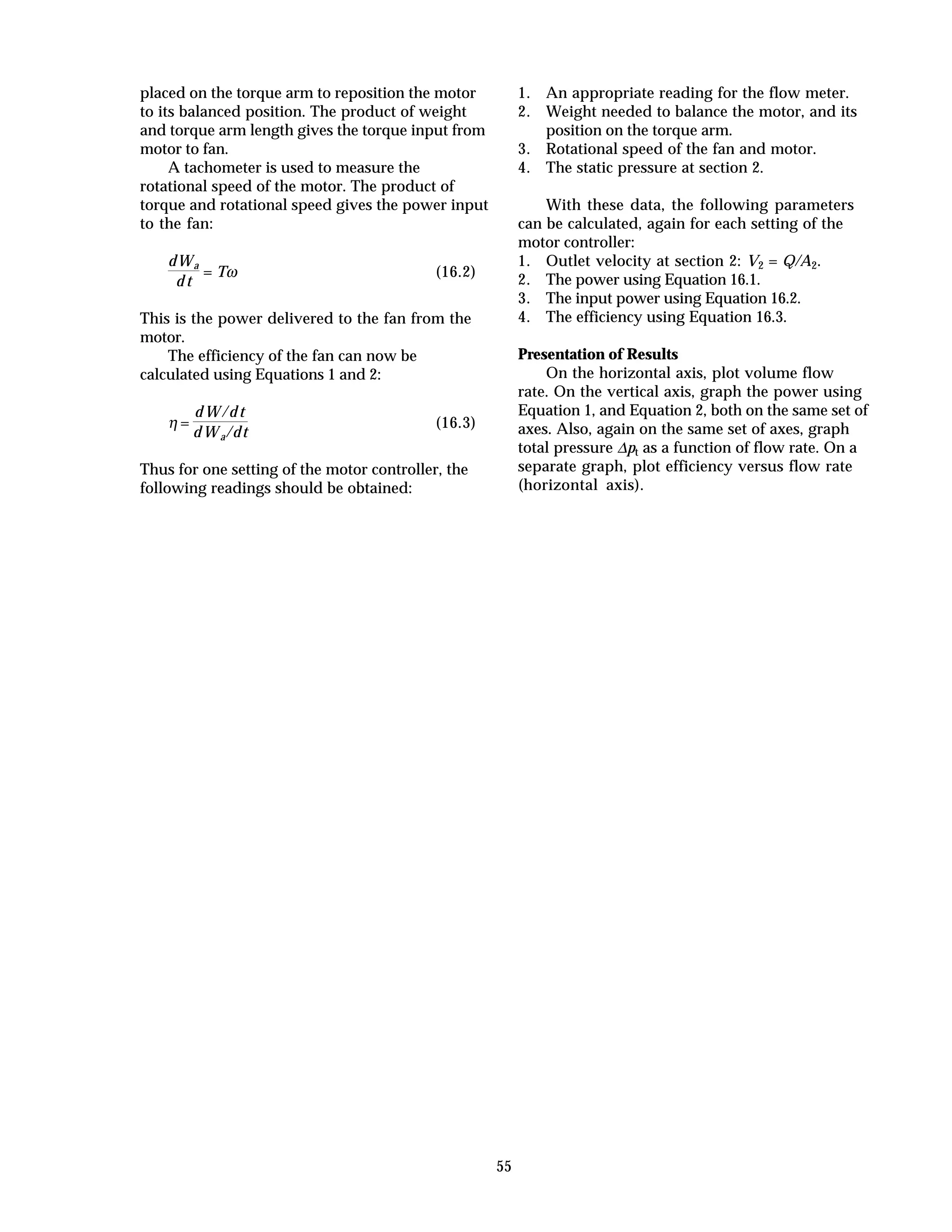
of an elbow meter is shown in Figure 19.1
flow
D
R
45o
pressure
tap
FIGURE 19.1. Schematic of an elbow meter
showing pressure tap locations.
Installation. It is necessary to select an elbow in a
line where flow rate is to be measured. The
internal dimensions of R and D must be known for
the elbow of interest. Holes are drilled in specific
locations as shown to accept 1/8th nominal pipe
threads or something different if desired.
Pressure measurements are made to determine
the pressure drop that exists as well as the
corresponding flow rate.
Theory. The pressure measurement devices are
attached to the connectors and flow through the
pipe is initiated. The difference in pressure
between the tap locations is to be determined.
As given in [1], the flow rate through the
meter can be calculated with:
Q = A K
√
R
D
∆ p
ρ
where
A = cross sectional area = πD2/4 in ft2
K= 1 -
6.5
√Re
= correction factor (19.1)
Re = Reynolds number = ρVD/µ
104 ≤ Re ≤ 106
ρ = fluid density in slug/ft3
µ = fluid viscosity in lbf·s/ft2
∆p = pressure drop in lbf/ft2
D = diameter in ft
R = radius of elbow in ft
Sample Calculation. Show how flow rate is
calculated using a 4 nominal schedule 80 short
radius elbow meter. Pressure is measured with a
manometer. Water is the working fluid.
Solution: For a 4 nominal, short radius elbow we
have [2]:
R = 4 in. = 0.333 ft D = 0.3198 ft
We calculate
A =
πD2
4
=
π(0.3198)2
4
= 0.0803 ft2
For water,
ρ = 1.94 slug/ft3 µ = 1.9 x 10⁻⁵ lbf·s/ft2
A calibration curve is one that relates the volume
flow rate through the meter to the pressure drop,
using whatever units are convenient. We are
calculating the calibration results for only one
data point in such a curve. In this example, we
measure flow rate in gpm, and because we are
using a manometer, we express pressure drop in](https://image.slidesharecdn.com/fluidslabmanual2-140524214604-phpapp01/75/Fluids-lab-manual_2-62-2048.jpg)
![63
terms of inches of water. A sample calculation for
a flow rate of, say, 150 gpm is as follows. We
have
Q = 150 gpm (2.229 x 10⁻³) = 0.334 ft3/s
The flow velocity then is
V =
Q
A
=
0.334
0.0803
= 4.16 ft/s
To find ∆p, we must first find K which in turn
depends on Reynolds number:
Re=
ρVD
µ
=
1.94(4.16)(0.3198)
1.9 x 10-5 = 1.36 x 10⁵
Then
K = 1 -
6.5
√Re
= 1 -
6.5
√1.36 x 105
= 0.982
For an elbow meter,
Q = A K
√
R
D
∆ p
ρ
Rearranging and solving for ∆p gives
∆p = ρ
Q
A K
2 D
R
(19.2)
Substituting
∆p = (1.94)
0.334
0.0803(0.982)
2 0.3198
0.333
or ∆p = 33.4 lbf/ft2
Now in terms of a column of water,
∆h =
∆p
ρg
=
33.4
1.94(32.2)
= 0.534 ft of water
or ∆h = 6.41 in. of water
For calculations of this type on an elbow that has
not been tested in the laboratory, the result is
accurate to within ± 4%. That is, for a reading ∆h
of 6.41 in. of water, the flow rate can be as high
as 156 gpm or as low as 144 gpm. Note that a
manometer is not readable to the nearest
hundredth of an inch. Typically a reading will be
to the nearest tenth of an inch.
So based on the results here, one data point on
the calibration curve is:
∆h = 6.4 in of water Q = 150 gpm
Calibration. In the preceding calculation, note
the dependence of the results on having an
equation for the correction factor K (Equation
19.1). The equation for K was derived from
theoretical considerations [1], but it is desirable
to have experimental results to determine a
“better” relationship for it. We could use
Equation 19.2 with experimental data to
determine K, which is the subject of this exercise.
Thus, if we had an apparatus that is set up
and ready to use, we could measure flow rate Q,
determine R and D from a handbook [2], calculate
A, and reduce Equation 19.2 to:
∆p = (a known constant) x
Q
K
2
(19.3)
Then with the apparatus, we could obtain ∆p vs
Q for a number of data points. Using Equation
19.3, we could then calculate K.
Experiment Design
1. Design an apparatus for making measurements
on an elbow meter. It is desired to have the
capability of making measurements on 3/4, 1 and
1 1/2 inch line sizes/elbows. A sketch of the
apparatus is required, showing:
a) what fluid is to be used
b) the prime mover for pumping the fluid
c) where the fluid is to be stored
d) an accurate method for determining actual
flow rate
2. Write a procedure for the operator(s) to follow
in order to obtain the desired data.
3. Write a theory section that leads the reader
through a sample calculation and shows
specifically how the correction factor K is
determined.
4. How many data points should be obtained so
that K can be determined with 95% confidence?
References
[1] Fluid Meters: Their Theory and Application,
6th edition, 1971, ASME, New York, page 75.
[2] (Perry’s Chemical Engineering Handbook, pg.
6-57.](https://image.slidesharecdn.com/fluidslabmanual2-140524214604-phpapp01/75/Fluids-lab-manual_2-63-2048.jpg)

This document provides instructions and guidelines for conducting experiments in a fluid mechanics laboratory. It begins with an overview of course learning outcomes, safety procedures, and expectations for cleaning the lab space. It then discusses proper experimental methodology, including defining hypotheses, designing experiments to test hypotheses, collecting accurate and precise measurements, and analyzing results. The document emphasizes minimizing errors and uncertainties in measurements. It provides definitions for key terms like error, uncertainty, accuracy, and precision when evaluating experimental data. Finally, it outlines the content and procedures for 20 specific fluid mechanics experiments that will be conducted.


![Chapter 3 static forces on surfaces [compatibility mode]](https://cdn.slidesharecdn.com/ss_thumbnails/chapter-3-static-forces-on-surfaces-compatibility-mode-160214035852-thumbnail.jpg?width=640&height=640&fit=bounds)


