Downloaded 187 times

![Prof. Dr. Atıl BULU31
52.2
938.0
52.2
2
sec29.4
52.2
2
1
1
2
1
2
1
1
2
1
21
=
′
+′
=
′
+′
=
==′
y
y
yg
q
y
mq
mEE c
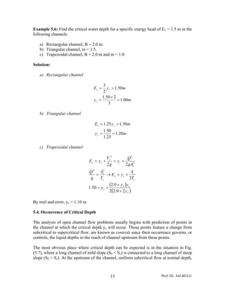
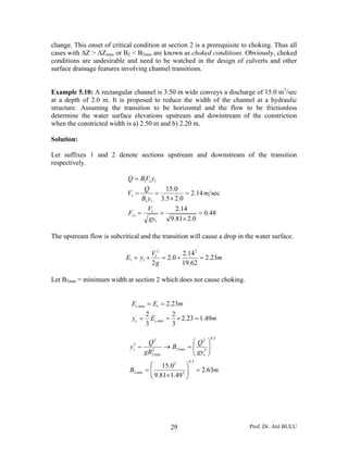
Solving by trial and error, the appropriate depth to give subcritical flow is,
my 35.21 =′
[Note that for the same discharge when B2 < B2min (i.e. under choking conditions) the
depth at the critical section will be different from yc = 1.49 m and depends on the value
B2].
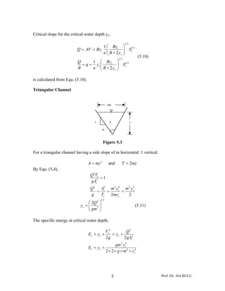
5.5.2.4. General Transition
A transition in general form may have a change of channel shape, provision of a hump or
a depression, contraction or expansion of channel width, in any combination. In addition,
there may be various degrees of loss of energy at various components. However, the
basic dependence of the depths of flow on the channel geometry and specific energy of
flow will remain the same. Many complicated transition situations can be analyzed by
using the principles of specific energy and critical depth.
In subcritical flow transitions the emphasis is essentially to provide smooth and gradual
changes in the boundary to prevent flow separation and consequent energy losses. The
transitions in supercritical flow are different and involve suppression of shock waves
related disturbances.
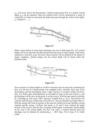
Example 5.12: A discharge of 16.0 m3
/sec flows with a depth of 2.0 m in a rectangular
channel 4.0 m wide. At a downstream section the width is reduced to 3.50 m and the
channel bed is raised by ΔZ. Analyze the water surface elevations in the transitions when
a) ΔZ = 0.20 m and b) ΔZ = 0.35 m.
Solution:
Let the suffixes 1 and 2 refer to the upstream and downstream sections respectively. At
the upstream section,
45.0
0.281.9
0.2
sec0.2
24
16
1
1
1
1
=
×
==
=
×
=
gy
V
F
mV
r](https://image.slidesharecdn.com/lecturenotes05-160123202502/85/Specific-Energy-Lecture-notes-05-31-320.jpg)
![Prof. Dr. Atıl BULU
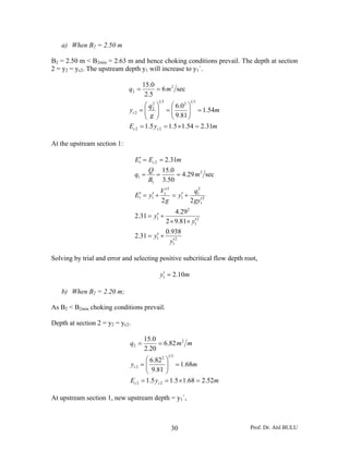
Since,
2
2
1
1 ,
y
q
V
y
q
VVyq ==→=
( ) ⎟⎟
⎠
⎞
⎜⎜
⎝
⎛
−+−=Δ 2
2
2
1
2
21
11
2 yyg
q
yyE (3)
It has been derived that,
( )
g
q
yyyy
2
2121
2
=+
( )2121
2
4
1
2
yyyy
g
q
+=
Putting this equation to Equation (3),
( ) ( )
( ) ( ) ( )
( ) ( ) ( )
( ) ( )[ ]
( )( )
21
2
1212
21
2
212112
21
12
2
212121
21
12
2
21
21
2
2
2
1
2
1
2
2
212121
4
4
4
4
4
4
1
)(
4
1
yy
yyyy
E
yy
yyyyyy
E
yy
yyyyyyyy
E
yy
yyyy
yyE
yy
yy
yyyyyyyE
−−
=Δ
++−−
=Δ
−++−
=Δ
−+
+−=Δ
−
++−=Δ
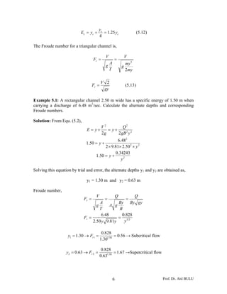
The analytical equation of the energy dissipated with the hydraulic jump is,
( )
21
3
12
4 yy
yy
E
−
=Δ (4)
The power lost by hydraulic jump can be calculated by,
EQN w Δ= γ
Where,
γw = Specific weight of water = 9.81 kN/m3
Q = Discharge (m3
/sec)
ΔE = Energy dissipated as head (m)
N = Power dissipated (kW)](https://image.slidesharecdn.com/lecturenotes05-160123202502/85/Specific-Energy-Lecture-notes-05-36-320.jpg)

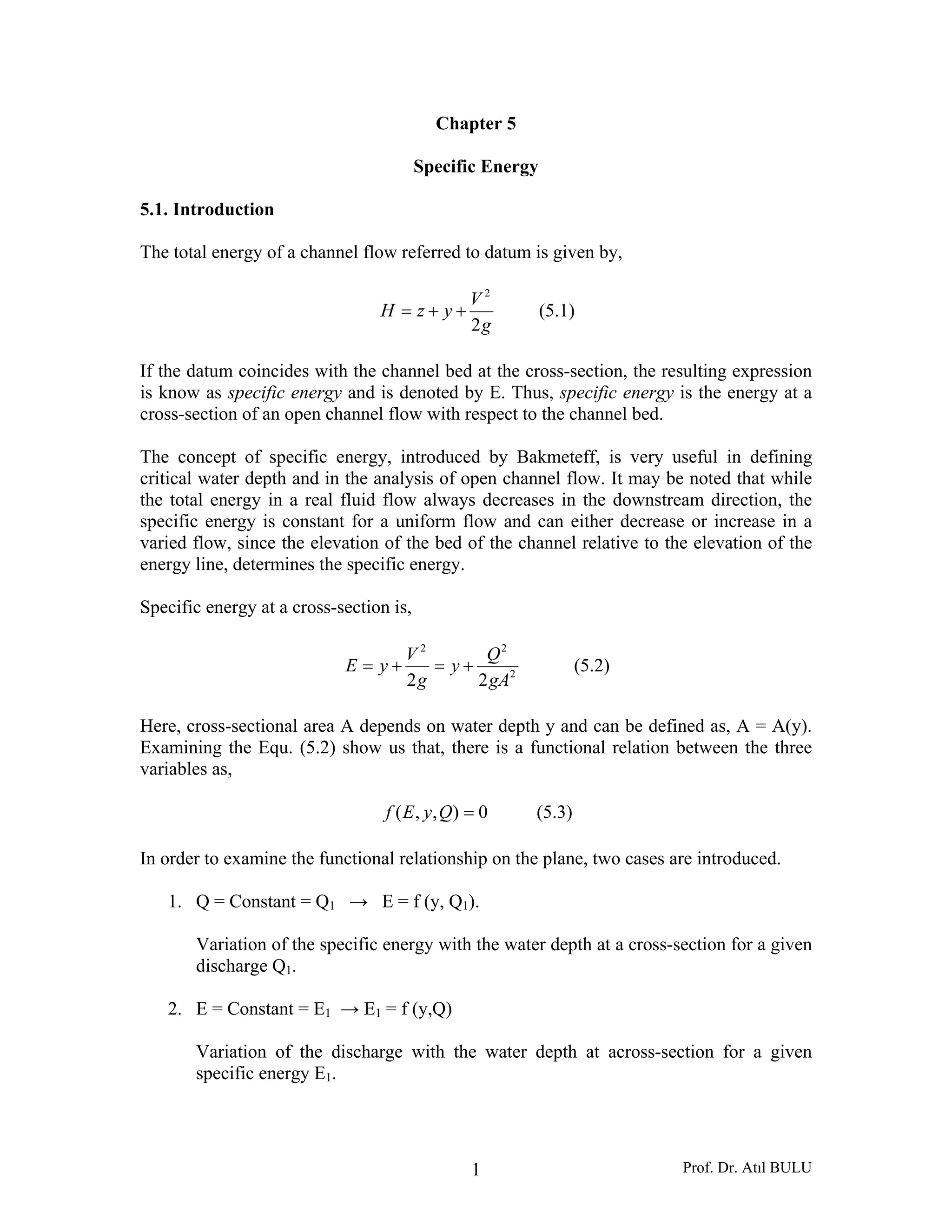
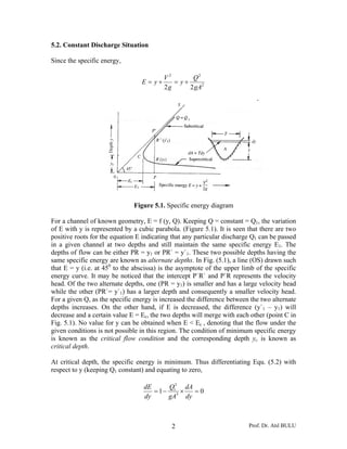
This document discusses specific energy in open channel flows. It defines specific energy as the total energy of a channel flow with respect to the channel bed. Specific energy is useful for analyzing critical flow conditions. For a given discharge, the variation of specific energy with depth forms a cubic parabola with two possible depths of flow (alternate depths). Critical flow occurs at the minimum specific energy where the two depths merge and the Froude number is 1. Equations are provided for calculating specific energy and critical flow properties in rectangular, triangular, and trapezoidal channel cross-sections. Examples demonstrate applying the equations to analyze specific energy, alternate depths, critical depth, and critical flow parameters.


![Unit 4[1]](https://cdn.slidesharecdn.com/ss_thumbnails/unit41-120525191354-phpapp02-thumbnail.jpg?width=640&height=640&fit=bounds)


