Download as PDF, PPTX
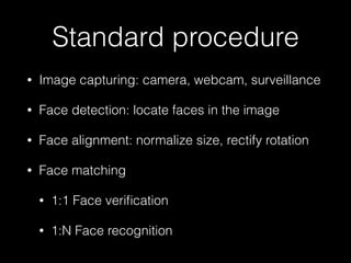
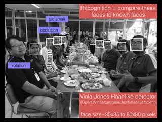

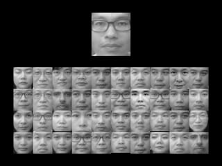


The document outlines the standard procedures and techniques used in face recognition and deep learning, including image capturing, face detection, alignment, and matching. It discusses various methods such as PCA, eigenfaces, and other advanced techniques to enhance recognition accuracy while addressing limitations like occlusion, lighting conditions, and pose variations. Deep learning developments in neural networks and applications like CNNs are also covered, emphasizing their importance in modern face recognition systems.


![[AI07] Revolutionizing Image Processing with Cognitive Toolkit](https://cdn.slidesharecdn.com/ss_thumbnails/ai07-170602095346-thumbnail.jpg?width=640&height=640&fit=bounds)