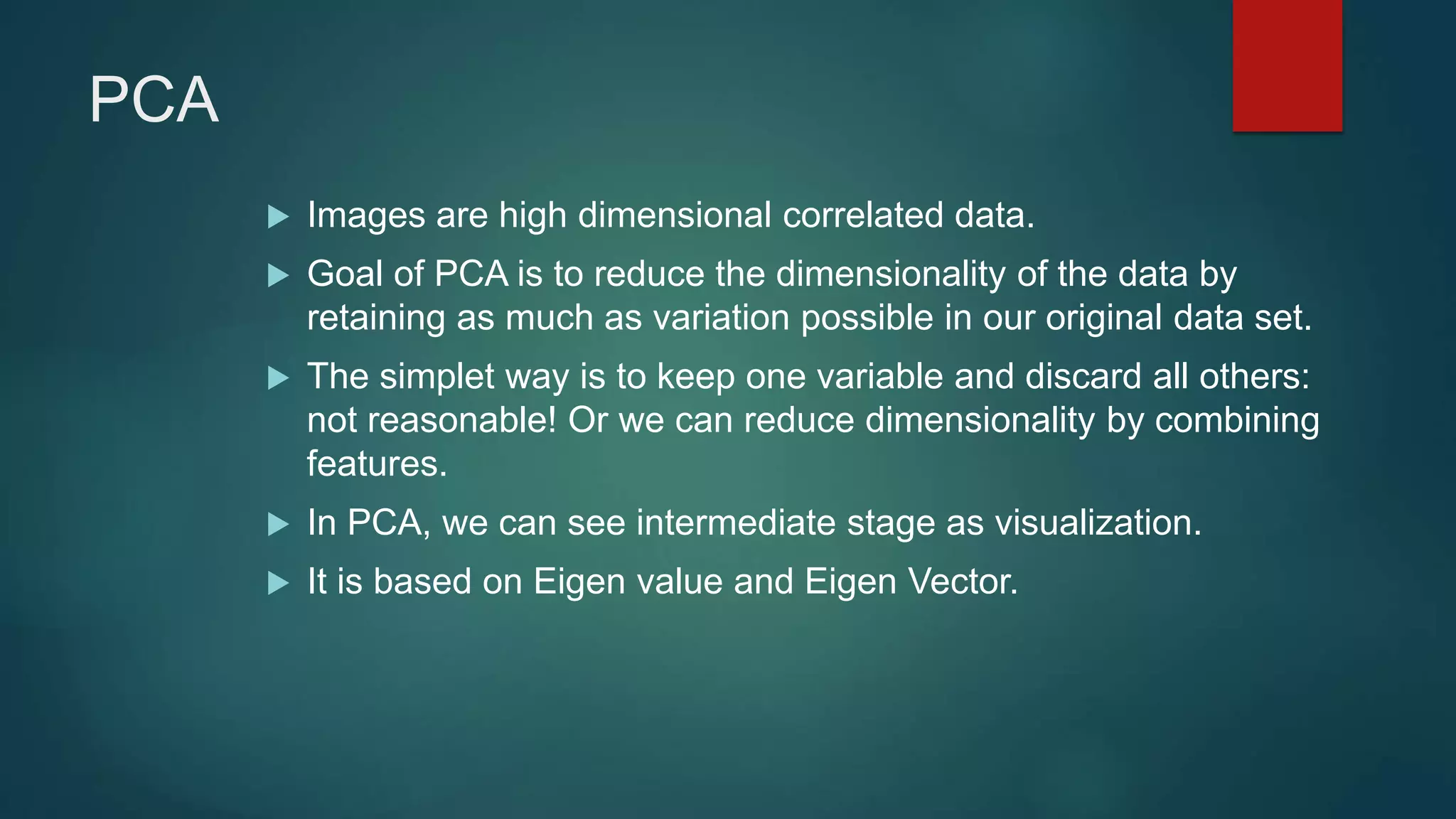
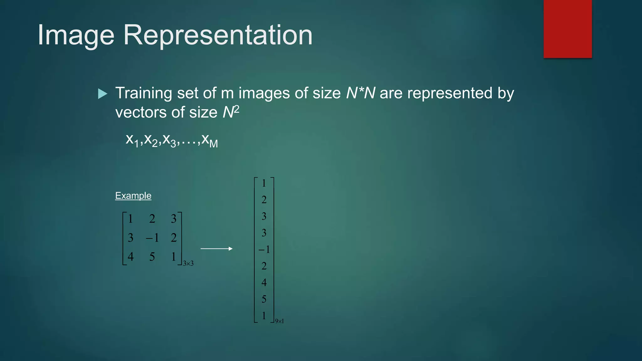
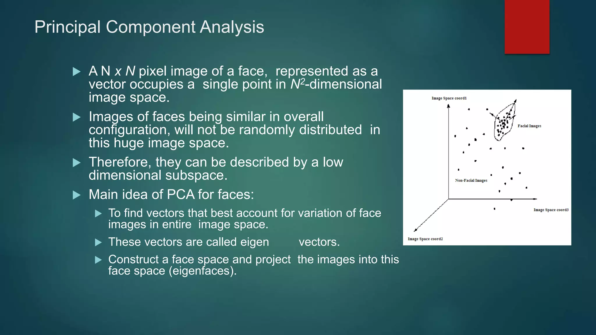
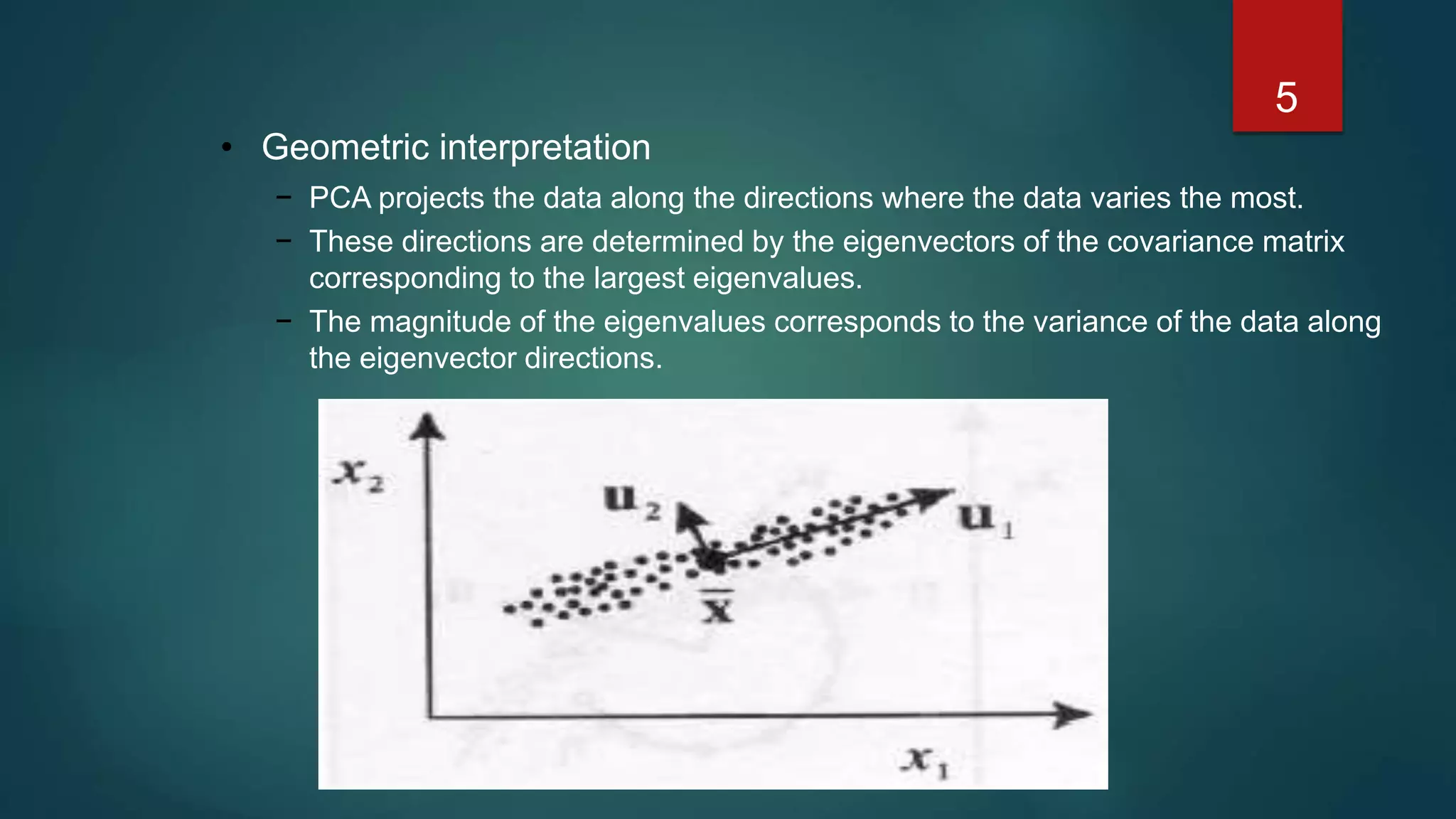
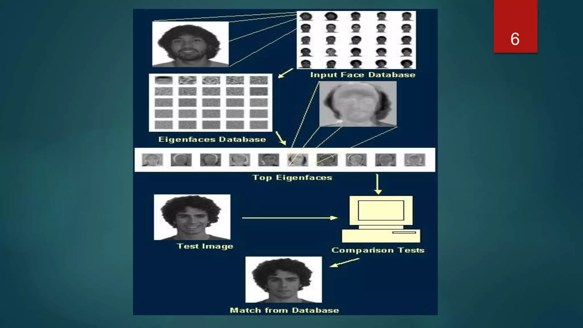
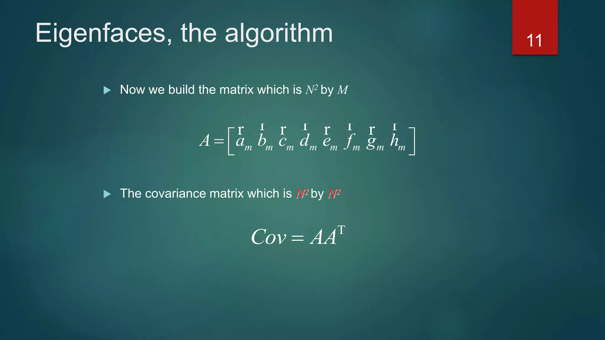
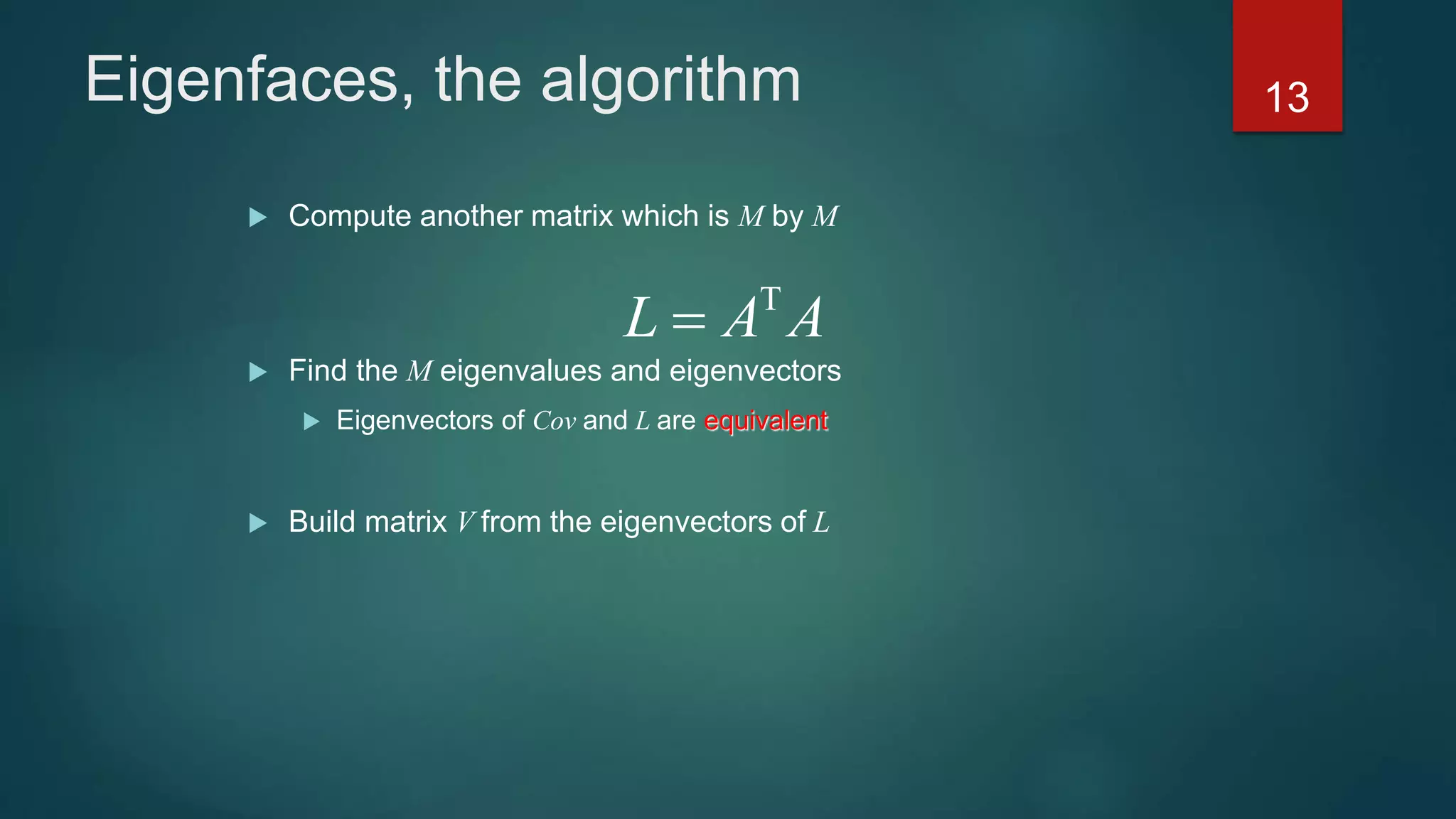
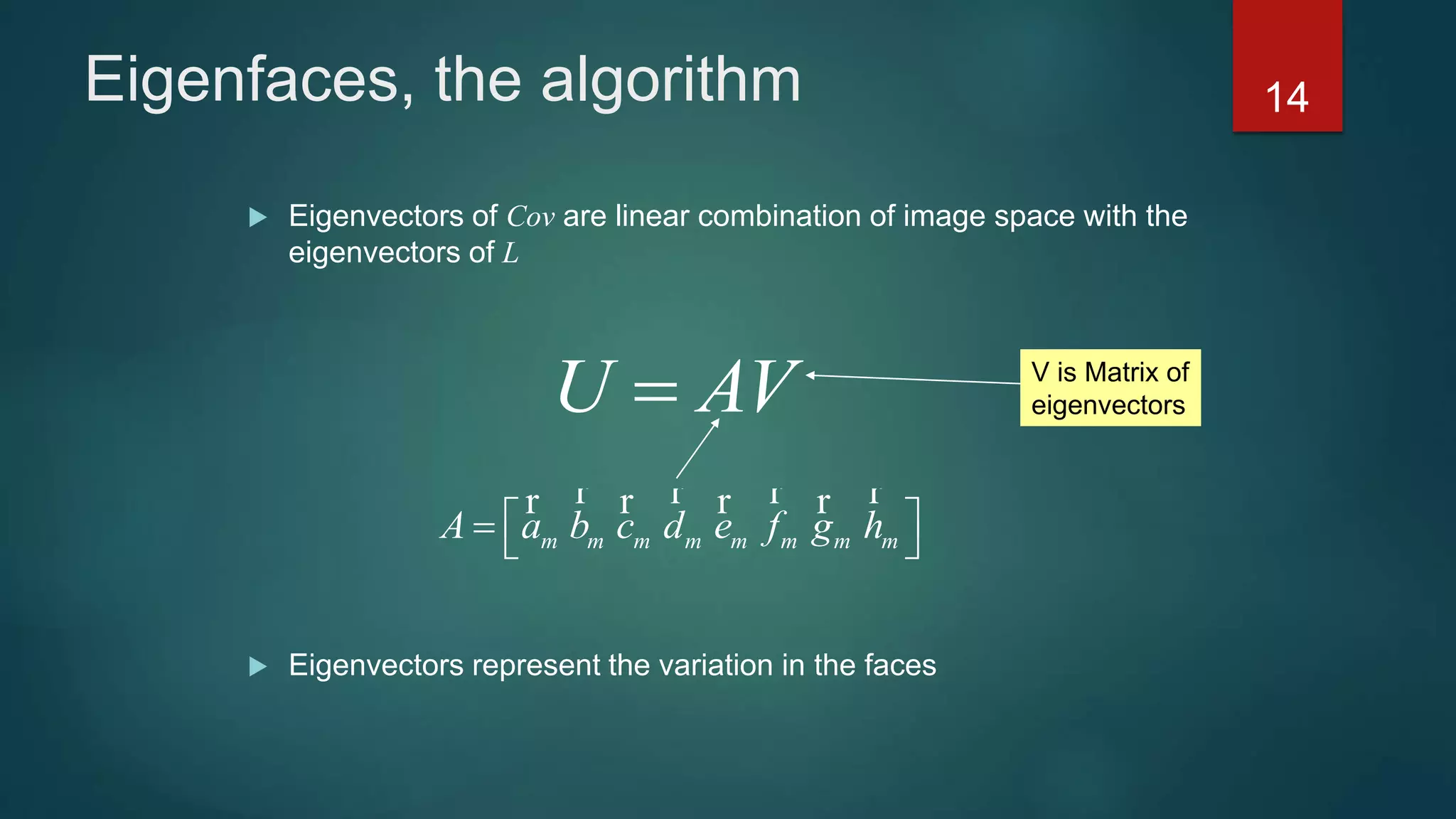
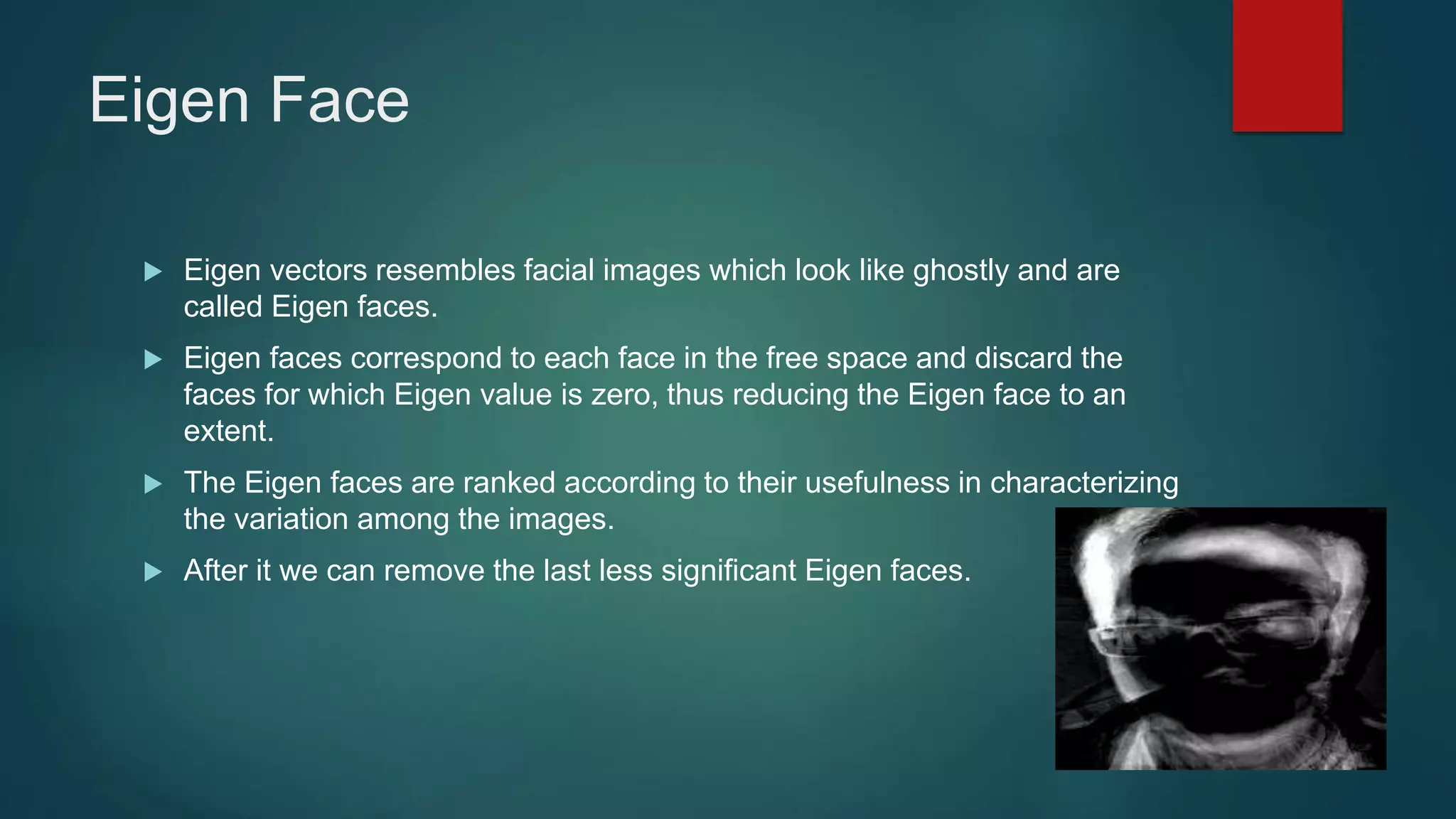
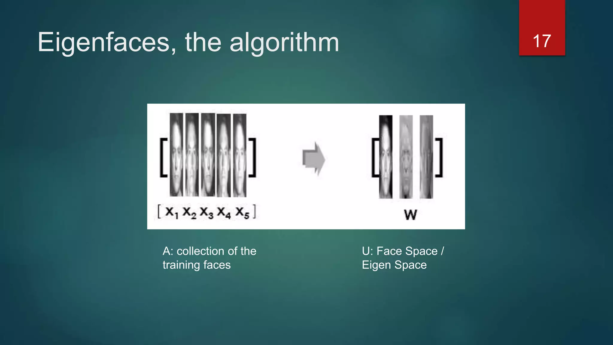
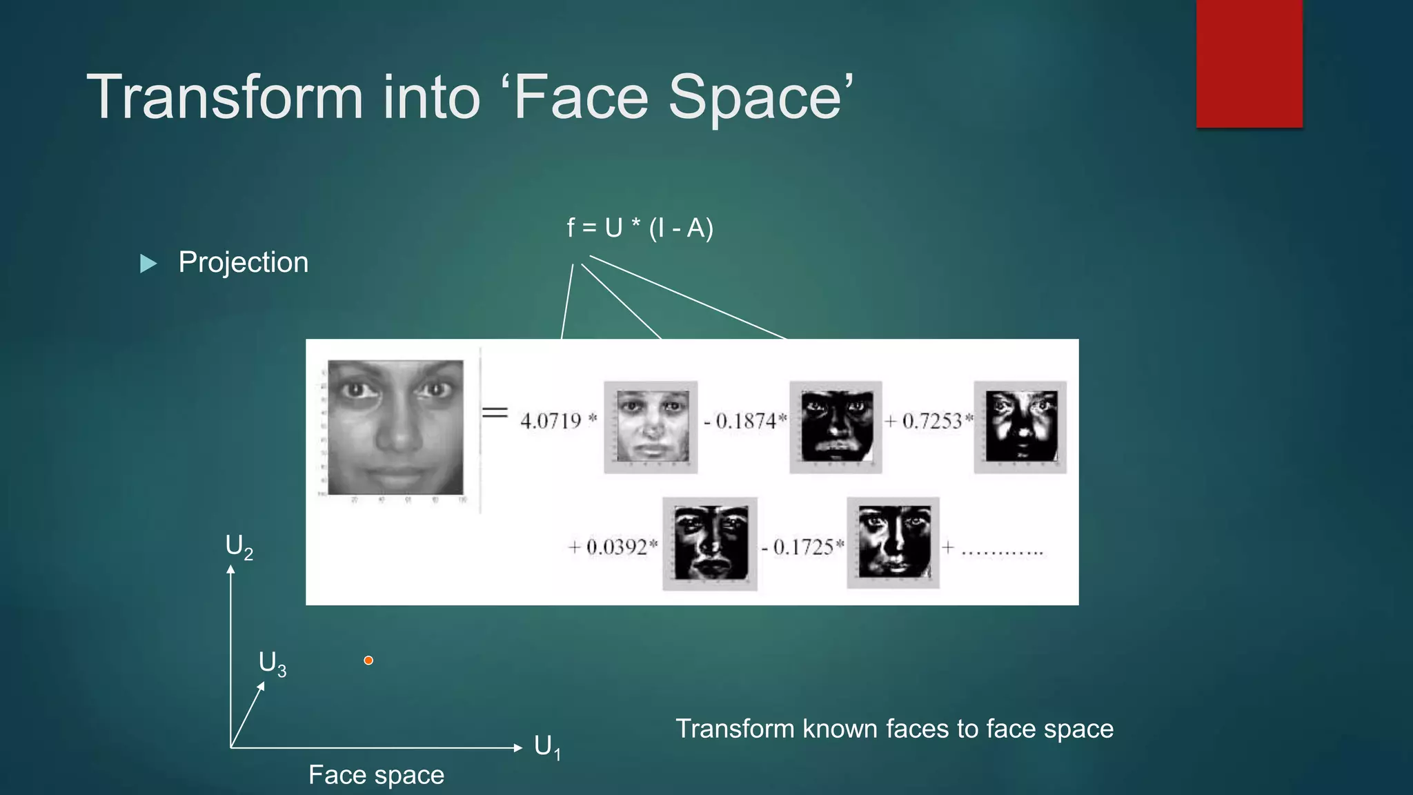
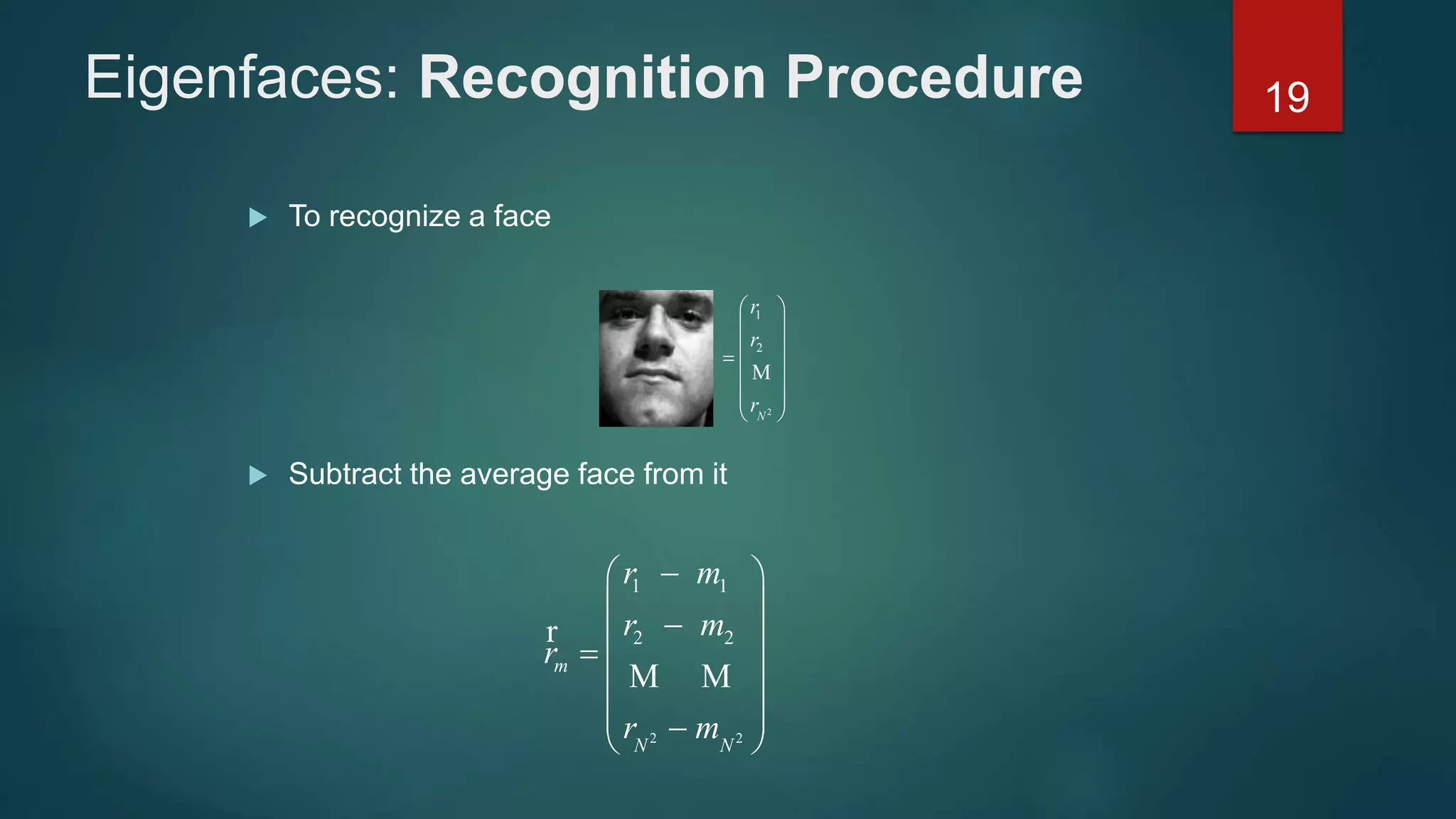
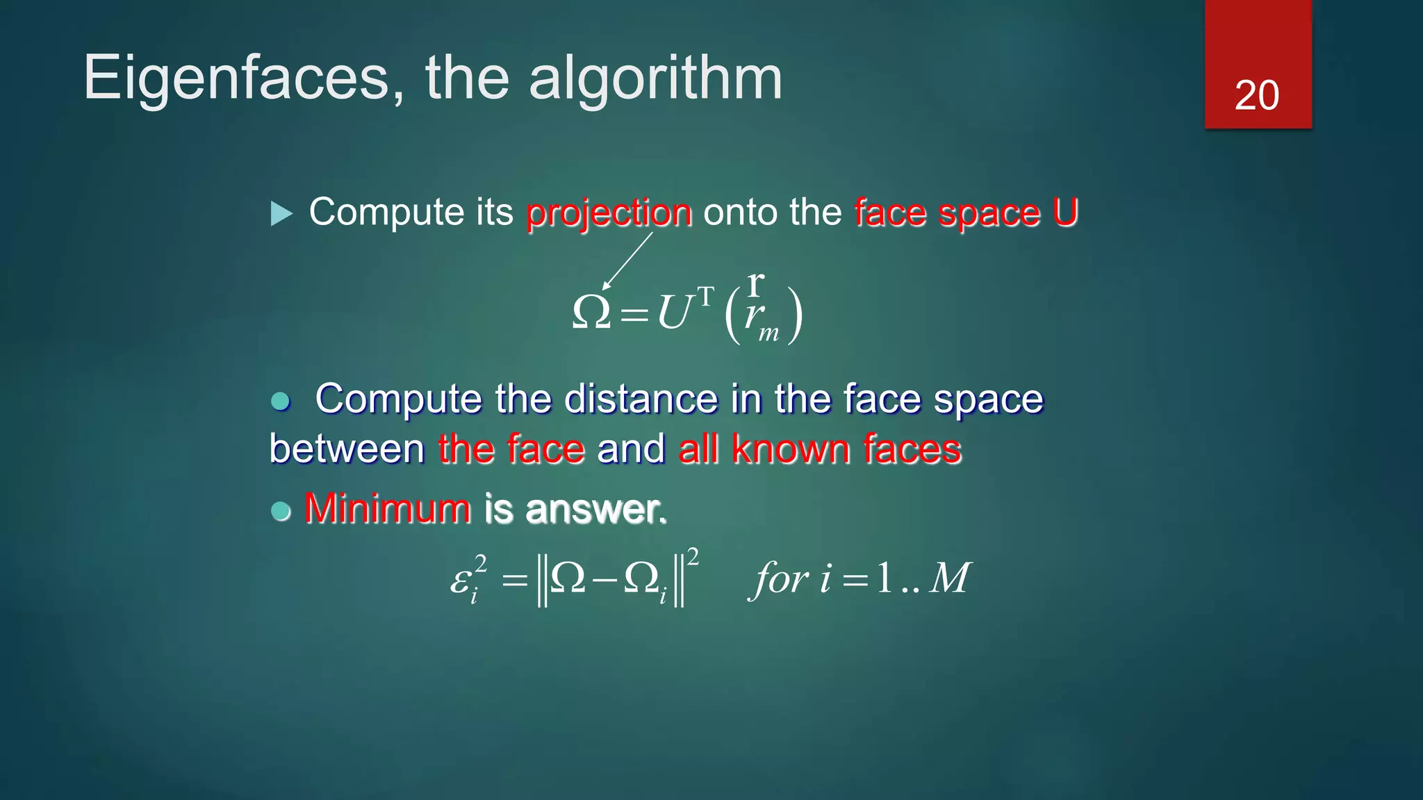
PCA is used to reduce the dimensionality of image data by finding the principal components that account for the most variance in the data. It works by constructing a feature space from the eigenvectors of the image covariance matrix. Images are represented as vectors in this lower-dimensional feature space rather than the original high-dimensional pixel space. The eigenvectors corresponding to the largest eigenvalues are the principal components or "eigenfaces" that best represent the variation between images. New images can be classified by projecting them into this eigenface feature space.

1. Principal component
analysis

2. PCA
 Images are high dimensional correlated data.
 Goal of PCA is to reduce the dimensionality of the data by
retaining as much as variation possible in our original data set.
 The simplet way is to keep one variable and discard all others:
not reasonable! Or we can reduce dimensionality by combining
features.
 In PCA, we can see intermediate stage as visualization.
 It is based on Eigen value and Eigen Vector.

3. Image Representation
 Training set of m images of size N*N are represented by
vectors of size N2
x1,x2,x3,…,xM
Example
33
154
213
321












19
1
5
4
2
1
3
3
2
1































4. Principal Component Analysis
 A N x N pixel image of a face, represented as a
vector occupies a single point in N2-dimensional
image space.
 Images of faces being similar in overall
configuration, will not be randomly distributed in
this huge image space.
 Therefore, they can be described by a low
dimensional subspace.
 Main idea of PCA for faces:
 To find vectors that best account for variation of face
images in entire image space.
 These vectors are called eigen vectors.
 Construct a face space and project the images into this
face space (eigenfaces).

5. 5
• Geometric interpretation
− PCA projects the data along the directions where the data varies the most.
− These directions are determined by the eigenvectors of the covariance matrix
corresponding to the largest eigenvalues.
− The magnitude of the eigenvalues corresponds to the variance of the data along
the eigenvector directions.

6. 6

7. Eigenfaces, the algorithm
 Assumptions
 Square images with Width = Height = N
 M is the number of images in the database
 P is the number of persons in the database
7

8. Eigenfaces, the algorithm
 The database
2
1
2
N
b
b
b
 
 
 
 
  
 
M
2
1
2
N
f
f
f
 
 
 
 
  
 
M
8
2
1
2
N
c
c
c
 
 
 
 
  
 
M
2
1
2
N
d
d
d
 
 
 
 
  
 
M
2
1
2
N
e
e
e
 
 
 
 
  
 
M
2
1
2
N
a
a
a
 
 
 
 
  
 
M
2
1
2
N
g
g
g
 
 
 
 
  
 
M
2
1
2
N
h
h
h
 
 
 
 
  
 
M

9. Eigenfaces, the algorithm
 We compute the average face
2 2 2
1 1 1
2 2 21
, 8
N N N
a b h
a b h
m where M
M
a b h
   
 
    
 
     
L
Lr
M M M
L
9

10. Eigenfaces, the algorithm
 Then subtract it from the training faces
 This reduce the common things to each face.
2 2 2 2 2 2 2 2
2 2
1 1 1 1 1 1 1 1
2 2 2 2 2 2 2 2
1 1 1 1
2 2
, , , ,
,
m m m m
N N N N N N N N
m m
N N
a m b m c m d m
a m b m c m d m
a b c d
a m b m c m d m
e m f m
e m f
e f
e m
          
       
             
       
                        
  
 
  
 
   
r rr r
M M M M M M M M
rr
M M
2 2 2 2 2 2
1 1 1 1
2 2 2 2 2 2
, ,m m
N N N N N N
g m h m
m g m h m
g h
f m g m h m
      
     
        
     
                 
rr
M M M M M M
10

11. Eigenfaces, the algorithm
 Now we build the matrix which is N2 by M
 The covariance matrix which is N2 by N2
m m m m m m m mA a b c d e f g h   
r r r rr r r r
Cov AA

11

12. Eigenfaces, the algorithm
 PCA assumes that the information is carried in the variance of the
features
 Find eigenvalues of the covariance matrix
 The matrix is very large
 The computational effort is very big
 We are interested in at most M eigenvalues
 We can reduce the dimension of the matrix
12

13. Eigenfaces, the algorithm
 Compute another matrix which is M by M
 Find the M eigenvalues and eigenvectors
 Eigenvectors of Cov and L are equivalent
 Build matrix V from the eigenvectors of L
L A A

13

14. Eigenfaces, the algorithm
 Eigenvectors of Cov are linear combination of image space with the
eigenvectors of L
 Eigenvectors represent the variation in the faces
U AV
m m m m m m m mA a b c d e f g h   
r r r rr r r r
14
V is Matrix of
eigenvectors

16. Eigen Face
 Eigen vectors resembles facial images which look like ghostly and are
called Eigen faces.
 Eigen faces correspond to each face in the free space and discard the
faces for which Eigen value is zero, thus reducing the Eigen face to an
extent.
 The Eigen faces are ranked according to their usefulness in characterizing
the variation among the images.
 After it we can remove the last less significant Eigen faces.

17. Eigenfaces, the algorithm 17
A: collection of the
training faces
U: Face Space /
Eigen Space

18. Transform into ‘Face Space’
 Projection
f = U * (I - A)
U1
U2
U3
Transform known faces to face space
Face space

19. Eigenfaces: Recognition Procedure
 To recognize a face
 Subtract the average face from it
2 2
1 1
2 2
m
N N
r m
r m
r
r m
 
 
 
 
   
r
M M
2
1
2
N
r
r
r
 
 
 
 
  
 
M
19

20. Eigenfaces, the algorithm
 Compute its projection onto the face space U
22
1..i i for i M   
20
 mU r
 
r
 Compute the distance in the face space
between the face and all known faces
 Minimum is answer.

21. 21• Problems
− Background (de-emphasize the outside of the face – e.g., by
multiplying the input image by a 2D Gaussian window centered on
the face)
− Lighting conditions (performance degrades with light changes)
− Scale (performance decreases quickly with changes to head size)
− Orientation (performance decreases but not as fast as with scale
changes)
− plane rotations can be handled
− out-of-plane rotations are more difficult to handle