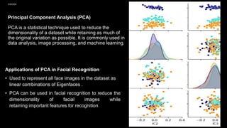
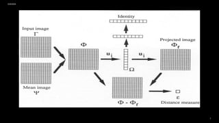
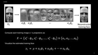
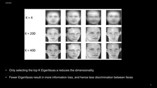
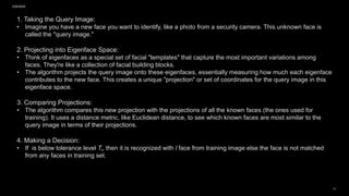
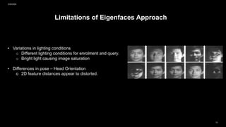
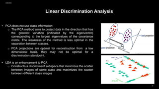
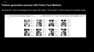
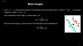
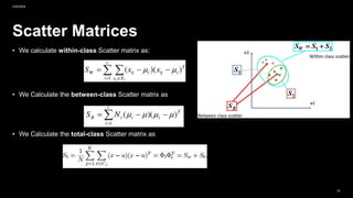
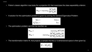
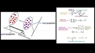
The document discusses face recognition methods, primarily focusing on eigenfaces and fisherfaces, which utilize statistical techniques like PCA and LDA for dimensionality reduction while improving classification accuracy. Eigenfaces are derived from covariance matrices of face images, while the fisherface method enhances PCA by maximizing class separation. The effectiveness of both algorithms is examined in terms of their application to face recognition, with fisherfaces showing superior performance under varying conditions.

1. 1
Eigenface , Fisherface
Face Recognition Methods

2. Introduction to Eigenfaces
What are Eigenfaces?
• Eigenfaces are the eigenvectors of the covariance matrix of the set of face images.
• They represent the most important features of a face.
2/20/2024
2

3. Principal Component Analysis (PCA)
PCA is a statistical technique used to reduce the
dimensionality of a dataset while retaining as much of
the original variation as possible. It is commonly used in
data analysis, image processing, and machine learning.
2/20/2024
Applications of PCA in Facial Recognition
• Used to represent all face images in the dataset as
linear combinations of Eigenfaces .
• PCA can be used in facial recognition to reduce the
dimensionality of facial images while
retaining important features for recognition
SAMPLE FOOTER TEXT 3

4. Eigenface Algorithm
2/20/2024
4
Overview
• The Eigenface algorithm is a facial
recognition technique used in computer
vision. It is based on the concept of
eigenvectors, which are used to reduce
the dimensionality of facial images while
preserving their important features.
Implementation
• The Eigenface algorithm works by first creating a set of
eigenvectors that represent the important features of facial
images. These eigenvectors are then used to create a new
set of images that are more easily recognizable by the
algorithm. The resulting images are then compared to a
database of known faces to identify matches.

5. PCA Method
• Face Image is represented as x(x,y) a 2dimension N by N array.
• If image size 256 by 256 this is equivalent to 65,536 dimension. Thus, this will be in 65,536-dimensional
space.
• The main idea of the principal component analysis is to find the vectors which best account for the distribution
of face images within the entire image space.
• We obtain the common face vector by summing up all the face vectors and divide them with the number of the
face vectors μ =
1
𝑚 𝑛=1
𝑚
𝑥𝑛 where (𝑥1, 𝑥2 ,…., 𝑥𝑛) are the face vectors.
• Then we Use the common Face vector to obtain the Unique face feature (Normalized) by 𝐴𝑛 = 𝑥𝑛 − μ.
• We obtain Eigen values and vectors using Covariance matrix by C =
1
𝑚 𝑛=1
𝑚
𝐴𝑛 𝐴𝑛
𝑇
• Compute each training image 𝑥𝑛 ‘s projections as 𝑋 → 𝑥𝑖
𝑐
⋅ 𝜙1, 𝑥𝑖
𝑐
⋅ 𝜙2, … , 𝑥𝑖
𝑐
⋅ 𝜙𝑘 ≡ 𝑎1, 𝑎2, … , 𝑎𝑘 .
• Visualize the estimated training face 𝑥𝑖 ≈ 𝜇 + 𝑎1𝜙1 + 𝑎2𝜙2 + ⋯ + 𝑎𝑘 𝜙𝑘 .
2/20/2024
5

6. 2/20/2024
6
The associated eigenvalues allow us to rank the eigenvectors according to their usefulness in characterizing the
variation among the images. Figure 2 shows the top seven Eigenfaces derived from the input images of Figure 1.
Figure two, Top Eigenfaces.
Figure one, Eigenfaces.

7. 2/20/2024
7

8. 2/20/2024
8
Compute each training image x i ‘s projections as
𝑋 → 𝑥𝑖
𝑐
⋅ 𝜙2, 𝑥𝑖
𝑐
⋅ 𝜙2, … , 𝑥𝑖
𝑐
⋅ 𝜙𝑘 ≡ 𝑎1, 𝑎2, … , 𝑎𝑘
Visualize the estimated training face
𝑥𝑖 ≈ 𝜇 + 𝑎1𝜙1 + 𝑎2𝜙2 + ⋯ + 𝑎𝑘 𝜙𝑘

9. 2/20/2024
9
• Only selecting the top K Eigenfaces a reduces the dimensionality.
• Fewer Eigenfaces result in more information loss, and hence less discrimination between faces

10. 2/20/2024
10

11. 2/20/2024
11
1. Taking the Query Image:
• Imagine you have a new face you want to identify, like a photo from a security camera. This unknown face is
called the "query image."
2. Projecting into Eigenface Space:
• Think of eigenfaces as a special set of facial "templates" that capture the most important variations among
faces. They're like a collection of facial building blocks.
• The algorithm projects the query image onto these eigenfaces, essentially measuring how much each eigenface
contributes to the new face. This creates a unique "projection" or set of coordinates for the query image in this
eigenface space.
3. Comparing Projections:
• The algorithm compares this new projection with the projections of all the known faces (the ones used for
training). It uses a distance metric, like Euclidean distance, to see which known faces are most similar to the
query image in terms of their projections.
4. Making a Decision:
• If is below tolerance level Tr, then it is recognized with l face from training image else the face is not matched
from any faces in training set.

12. 2/20/2024
12
Limitations of Eigenfaces Approach
• Variations in lighting conditions
o Different lighting conditions for enrolment and query.
o Bright light causing image saturation
• Differences in pose – Head Orientation
o 2D feature distances appear to distorted.

13. Fisherface
2/20/2024
• This method is a combination of PCA and LDA methods.
• Dimensionality reduction technique
• Maximizes separation between different classes in the
feature space
• Improves classification accuracy of eigenfaces
1
3

14. 2/20/2024
14
• PCA does not use class information
o The PCA method aims to project data in the direction that has
the greatest variation (indicated by the eigenvector)
corresponding to the largest eigenvalues of the covariance
matrix. The weakness of the method is less optimal in the
separation between classes.
o PCA projections are optimal for reconstruction from a low
dimensional basis, they may not be optimal for a
discrimination standpoint.
• LDA is an enhancement to PCA
o Constructs a discriminant subspace that minimizes the scatter
between images of same class and maximizes the scatter
between different class images
Linear Discrimination Analysis

15. • Fisherface is one of the popular algorithms used in face recognition and is widely believed to be superior to
other techniques, such as eigenface because of the effort to maximize the separation between classes in the
training process[1].
• This method is a combination of PCA and LDA methods. The PCA method is used to solve singular problems by
reducing the dimensions before being used to perform the LDA process. But the weakness of this method is that
when the PCA dimension reduction process will cause some loss of discriminant information useful in the LDA
process.
• The face image to be used must go through the preprocessing stage first. This stage includes image acquisition,
and RBG image conversion to grayscale.
• Fisherface method is a method that is a merger between PCA and LDA methods [1].
2/20/2024
15

16. 2/20/2024
How LDA Works ?
• LDA works by finding a linear combination of the original features that maximizes the separation between the
classes. Transform the original features into a new set of features that are more easily separable by a linear
classifier.
• The discriminant coefficients are computed using a linear regression model, where the dependent variable is
the class label, and the independent variables are the original features. The coefficients are then used to
transform the original features into a new set of features that are more easily separable by a linear classifier.
• LDA is often used as a preprocessing step in machine
learning algorithms, as it can significantly reduce the
dimensionality of a dataset while preserving class
separability. This can improve the performance of the
algorithm by reducing over fitting and improving
generalization.
Dimensionality Reduction

17. Feature generation process with Fisher Face Method :
2/20/2024
17
Assume that : Size of rectangular face image with height = N and width = N and consist of h samples image.

18. Mean Images
• Let 𝑋1, 𝑋2,…, 𝑋𝑐 be the face classes in the database and let each face class 𝑋𝑖, where i = 1,2,3,….,c has facial
images 𝑋𝑗, where j =1,2,3,…,k.
• We compute the mean image 𝜇𝑖 of each class 𝑋𝑖 as:
𝜇𝑖 =
1
𝑘 𝑗=1
𝑘
𝑋𝑗
• Now the mean image 𝜇𝑖 of all the class in the data base can be calculated as
𝜇=
1
𝑐 𝑖=1
𝑐
𝜇𝑖
2/20/2024
18

19. Scatter Matrices
• We calculate within-class Scatter matrix as:
• We Calculate the between-class Scatter matrix as
• We Calculate the total-class Scatter matrix as
2/20/2024
19

20. 2/20/2024
20
• Fisher’s classic algorithm now looks for a projection W, that maximizes the class separability criterion:
• A solution for this optimization problem is given by solving the General Eigenvalue Problem:
• The optimization problem can then be rewritten as:
• The transformation matrix W, that projects a sample into the (c-1)-dimensional space is then given by:

21. 2/20/2024
21

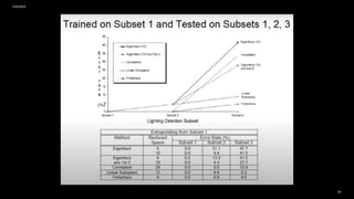
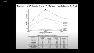
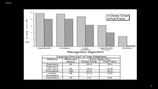
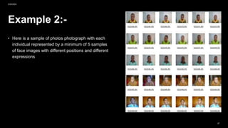
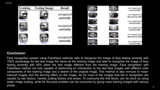
22. Example 1:-
2/20/2024
• A group of pictures were analyzed using
different methods like (Eigenface –
Correlation - Linear Subspace –
Fisherface) to show the accuracy of each
method.
• This is done by using pictures with
difference lighting positions to see which
is more accurate in different conditions
using different data.
• The Yale database is available for
download from http://cvc.yale.edu [3].
SAMPLE FOOTER TEXT 23

23. 2/20/2024
24

24. 2/20/2024
25

25. 2/20/2024
26

26. Example 2:-
• Here is a sample of photos photograph with each
individual represented by a minimum of 5 samples
of face images with different positions and different
expressions
2/20/2024
27

27. 2/20/2024
28
Face recognition system using Fisherface methods able to recognize the image of face testing correctly with
100% percentage for the test image the same as the training image and able to recognize the image of face
testing correctly with 93% when the test image different from the training image. Face recognition with
Fisherface method not only capable of performing an introduction to the test face images with different color
components of the training image and a sketch of the original image. This method is also immune to noise-
induced images and the blurring effect on the image. As for most of the images that fail in recognition are
caused by two factors, namely scaling factors and poses. To overcome the first factor, can be done by using
better image scaling, while for the pose problem can be overcome by giving more training images with various
poses.
Conclusion

28. Reference :
2/20/2024
29
1. Anggo, M., & Arapu, L. (2018). Face Recognition Using Fisherface Method. Journal of Physics.
Conference Series, 1028, 012119. https://doi.org/10.1088/1742-6596/1028/1/012119
2. Turk, M. A., & Pentland, A. P. (2002). Face recognition using eigenfaces. Proceedings. 1991 IEEE
Computer Society Conference on Computer Vision and Pattern Recognition.
3. Belhumeur, P. N., Hespanha, J. P., & Kriegman, D. J. (1997). Eigenfaces vs. Fisherfaces: recognition
using class specific linear projection. IEEE Transactions on Pattern Analysis and Machine
Intelligence, 19(7), 711–720. https://doi.org/10.1109/34.598228
4. Eigenfaces for Recognition by: M. A. Turk, A. P. Pentland. Journal of Cognitive Neuroscience, Vol. 3,
No. 1. (1991), pp. 71-86.

29. Crew Group 14:
• Mostafa Younes Mostafa (120210289) Section(4)
• Karim Walid Fathy (120210220) Section(3)
2/20/2024
30
Egypt Japan University Of Science & Technology