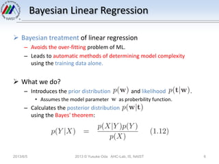
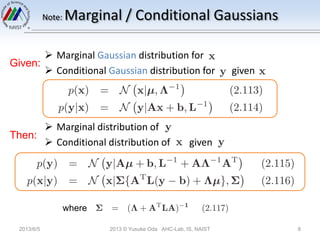
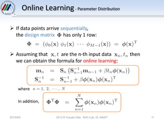
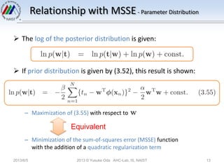
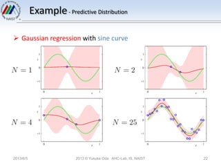
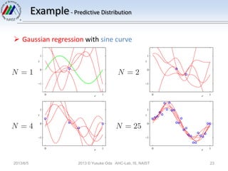
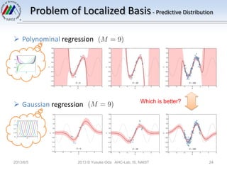
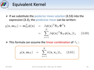
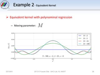
Pattern Recognition and Machine Learning: Section 3.3

Reading
Pattern Recognition
and Machine Learning
§3.3 (Bayesian Linear Regression)
Christopher M. Bishop
Introduced by: Yusuke Oda (NAIST)
@odashi_t
2013/6/5 2013 © Yusuke Oda AHC-Lab, IS, NAIST 1

Agenda
 3.3 Bayesian Linear Regression ベイズ線形回帰
– 3.3.1 Parameter distribution パラメータの分布
– 3.3.2 Predictive distribution 予測分布
– 3.3.3 Equivalent kernel 等価カーネル

Agenda

Bayesian Linear Regression
 Maximum Likelihood (ML)
– The number of basis functions (≃ model complexity)
depends on the size of the data set.
– Adds the regularization term to control model complexity.
– How should we determine
the coefficient of regularization term?

 Maximum Likelihood (ML)
– Using ML to determine the coefficient of regularization term
... Bad selection
• This always leads to excessively complex models (= over-fitting)
– Using independent hold-out data to determine model complexity
(See §1.3)
... Computationally expensive
... Wasteful of valuable data
In the case of previous slide,
λ always becomes 0
when using ML to determine λ.

 Bayesian treatment of linear regression
– Avoids the over-fitting problem of ML.
– Leads to automatic methods of determining model complexity
using the training data alone.
 What we do?
– Introduces the prior distribution and likelihood .
• Assumes the model parameter as proberbility function.
– Calculates the posterior distribution
using the Bayes' theorem:

Agenda

Note: Marginal / Conditional Gaussians
 Marginal Gaussian distribution for
 Conditional Gaussian distribution for given
 Marginal distribution of
 Conditional distribution of given
Given:
Then:
where

Parameter Distribution
 Remember the likelihood function given by §3.1.1:
– This is the exponential of quadratic function of
 The corresponding conjugate prior is given by
a Gaussian distribution:
known parameter

Parameter Distribution
 Now given:
 Then the posterior distribution is shown by using (2.116):
where

Online Learning- Parameter Distribution
 If data points arrive sequentially,
the design matrix has only 1 row:
 Assuming that are the n-th input data then
we can obtain the formula for online learning:
where
In addition,

Easy Gaussian Prior- Parameter Distribution
 If the prior distribution is a zero-mean isotropic Gaussian
governed by a single precision parameter :
 The corresponding posterior distribution is also given:
where

Relationship with MSSE- Parameter Distribution
 The log of the posterior distribution is given:
 If prior distribution is given by (3.52), this result is shown:
– Maximization of (3.55) with respect to
– Minimization of the sum-of-squares error (MSSE) function
with the addition of a quadratic regularization term
Equivalent

Example- Parameter Distribution
 Straight-line fitting
– Model function:
– True function:
– Error:
– Goal: To recover the values of
from such data
– Prior distribution:

Generalized Gaussian Prior- Parameter Distribution
 We can generalize the
Gaussian prior about exponent.
 In which corresponds
to the Gaussian
and only in the case is the
prior conjugate to the (3.10).

Agenda

Predictive Distribution
 Let's consider that making predictions of directly
for new values of .
 In order to obtain it, we need to evaluate the
predictive distribution:
 This formula is tipically written:
Marginalization arround
(summing out )

 The conditional distribution of the target variable is given:
 And the posterior weight distribution is given:
 Accordingly, the result of (3.57) is shown by using (2.115):
where

 Now we discuss the variance of predictive distribution:
– As additional data points are observed, the posterior distribution
becomes narrower:
– 2nd term of the(3.59) goes zero in the limit :
Addictive noise
goverened by the parameter .
This term depends on the mapping vector
. of each data point .

Example- Predictive Distribution
 Gaussian regression with sine curve
– Basis functions: 9 Gaussian curves
Mean of predictive distribution
Standard deviation of
predictive distribution

Problem of Localized Basis- Predictive Distribution
 Polynominal regression
 Gaussian regression
Which is better?

 If we used localized basis function such as Gaussians,
then in regions away from the basis function centers
the contribution from the 2nd term in the (3.59) will goes zero.
 Accordingly, the predictive variance becomes only the noise
contribution . But it is not good result.
Large contribution
Small contribution

 This problem (arising from choosing localized basis function)
can be avoided by adopting an alternative Bayesian approach
to regression known as a Gaussian process.
– See §6.4.

Case of Unknown Precision- Predictive Distribution
 If both and are treated as unknown then
we can introduce a conjugate prior distribution and
corresponding posterior distribution as Gaussian-gamma
distribution:
 And then the predictive distribution is given:

Agenda

Equivalent Kernel
 If we substitute the posterior mean solution (3.53) into the
expression (3.3), the predictive mean can be written:
 This formula can assume the linear combination of :

Equivalent Kernel
 Where the coefficients of each are given:
 This function is calld smoother matrix or equivalent kernel.
 Regression functions which make predictions by taking linear
combinations of the training set target values are known as
linear smoothers.
 We also predict for new input vector using equivalent
kernel, instead of calculating parameters of basis functions.

Example 1- Equivalent Kernel
 Equivalent kernel with Gaussian regression
 Equivalen kernel depends on the set of basis function and the
data set.

Equivalent Kernel
 Equivalent kernel means the contribution of each data point
for predictive mean.
 The covariance between and can be shown by
equivalent kernel:
Large contribution
Small contribution

Properties of Equivalent Kernel- Equivalent Kernel
 Equivalent kernel have localization property even if any basis
functions are not localized.
 Sum of equivalent kernel equals 1 for all :
Polynominal Sigmoid

 Equivalent kernel with polynominal regression
– Moving parameter:

Properties of Equivalent Kernel- Equivalent Kernel
 Equivalent kernel satisfies an important property shared by
kernel functions in general:
– Kernel function can be expressed in the form of an inner product with
respect to a vector of nonlinear functions:
– In the case of equivalent kernel, is given below:

Thank you!
zzz...

Pattern Recognition and Machine Learning: Section 3.3

More Related Content

What's hot

Viewers also liked

Similar to Pattern Recognition and Machine Learning: Section 3.3

More from Yusuke Oda

Recently uploaded

Pattern Recognition and Machine Learning: Section 3.3