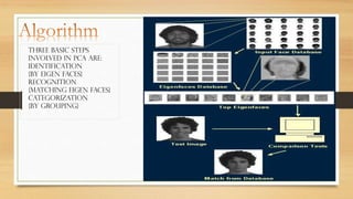
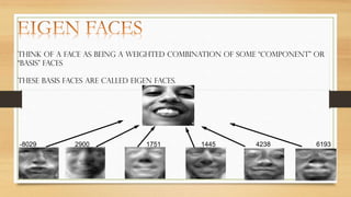
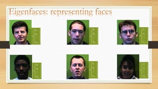
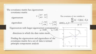
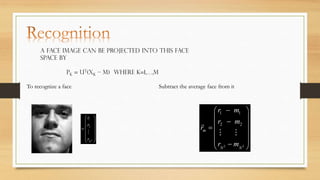
PCA is used for face recognition. It involves calculating eigenvectors from a training set of face images to define a feature space called "eigenfaces". A new face is recognized by projecting it onto this space and comparing to existing faces. PCA works by identifying directions of maximum variance in the training data, capturing the most important information about faces with fewer vectors. Potential applications include identification, security, and human-computer interaction. However, it is sensitive to changes in lighting and expression.

1. Face recognition using PCA
R.SINDHI MADHURI
A.ANURAG REDDY
G.USHASWI
ROHIT UPADHYAY

2. •
•
•
•
•
IDEA
OPERATIONS
MERITS
DEMERITS
APPLICATIONS

3. PCA
Eigenfaces: the idea
Eigenvectors and Eigenvalues
Learning Eigenfaces from training sets of faces
Co-variance
Recognition and reconstruction

4. PCA means Principle Component Analysis.
PCA was invented in 1901 by Karl Pearson
PCA involves the calculation of the eigenvalue
decomposition of a data covariance matrix or
singular value decomposition of a data matrix,
usually after mean centering the data for each
attribute.

5. Three basic steps
involved in PCA are:
Identification
{by eigen faces}
Recognition
{matching eigen faces}
Categorization
{by grouping}

6. In Digital Image Processing, we convert 2-D images into matrix form for clear analysis.
Every matrix can be represented with the help of its eigen vectors.
An eigenvector is a vector that obeys the following rule:
Av   v
Where A is a matrix , is a scalar (called the eigenvalue)
e.g. A   2
3 one eigenvector of is
 3  since
  
 2 1


2
 2 3  3 12
3
 2 1  2    8   4   2 

   
 
so for this eigenvector of this matrix the eigenvalue is 4

7. Think of a face as being a weighted combination of some “component” or
“basis” faces
These basis faces are called eigen faces.
-8029
2900
1751
1445
4238
6193

8.  a1 


a2 




a 2 

 N 
 d1 


 d2 




d 2 

 N 
 b1 


b2 




b 2 

 N 
 c1 


c2 




c 2 

 N 
 e1 


e2 




e 2 

 N 
 f1 


 f2 




f 2

 N 

9. We compute the average face
 a1  b1 

1  a2  b2 
m
M

a 2 b 2 
N
 N
 h1 

 h2 
,


 hN 2 

where M  8

10. Then subtract it from the training faces
 a1  m1 
 b1  m1 
 c1  m1 
 d1  m1 








 a2  m2  , b   b2  m2  , c   c2  m2  , d   d 2  m2  ,
am 
m
m
m












a 2  m 2 

b 2  m 2 

c 2  m 2 

d 2  m 2 

N 
N 
N 
N 
 N
 N
 N
 N
 e1  m1 


e2  m2 
em  
,



e 2  m 2 

N 
 N
 f1  m1 
 g1  m1 
 h1  m1 






f 2  m2 
g 2  m2 
h2  m2 
fm  
, gm  
, hm  









f 2 m 2

g 2  m 2 

h 2  m 2 

N 
N 
N 
 N
 N
 N

11. Now we build the matrix which is N2 by M
A   am bm cm d m em f m g m hm 


The covariance matrix which is N2 by N2

Cov  AA

12. The covariance matrix has eigenvectors
covariance matrix
eigenvectors
eigenvalues
.617 .615 
C

.615 .717 
 .735

 .678 
1  
The covariance of two variables is:
n
.678
2  
.735


Eigenvectors with larger eigenvectors correspond to
1  0.049
2  1.284
directions in which the data varies more
Finding the eigenvectors and eigenvalues of the
covariance matrix for a set of data is termed
principle components analysis
cov( x1 , x2 ) 
i
( x1i  x1 )( x2 x2 )

i 1
n 1

13. A face image can be projected into this face
space by
pk = UT(xk – m) where k=1,…,m
To recognize a face
Subtract the average face from it
 r1 
 
r2
 
 
 
r 2 
 N 
 r1  m1 


r2  m2 
rm  



r 2  m 2 

N 
 N

14. Compute its projection onto the face space U
 U
Compute the distance in the face  2
i
space between the face and all
known faces
Compute the threshold


 rm 
   i
1
  max i   j
2
2
for i  1.. M
 for i, j  1.. M

15. Distinguish between
• If    then it’s not a face; the distance between
the face and its reconstruction is larger than
threshold
• If    and min  i    then it’s a new face
• If    and  i   , (i  1.. M ) then it’s a known
face because the distance in the face space
between the face and all known faces is larger than
threshold

16. Image is reconstructed in the 3rd case, if
   and 
i
  , (i  1.. M )
Using the MATLAB code, original image and reconstructed image are shown.
Ex:

17. Relatively simple
Fast
Robust
Expression
- Change in feature
location and shape.

18. Variations in lighting
conditions
Different lighting conditions
for enrolment and query.
Bright light causing image
saturation.

19. Various potential
applications, such as
•
•
Person identification.
Human-computer
interaction.
• Security systems.