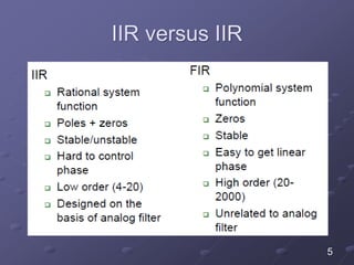
The document details the filter design process, highlighting three main steps: selecting appropriate filter design techniques based on desired characteristics, choosing between FIR and IIR filters based on phase distortion tolerance and complexity, and specifying discrete-time filter designs from continuous-time analog filters. It discusses methods for determining filter coefficients and emphasizes the stability and causality in filter design, alongside practical issues such as aliasing. The document also covers specific examples of designing filters using methods like impulse invariance and bilinear transformation.

1. Filter design process
In general the design of filter is composed
from three different steps
1

2. Filter design techniques
In the design of frequency selective filters,
the desired filter characteristics are
specified in the frequency domain in terms
of the desired magnitude and phase
response of the filter
In the filter design process, we determine
the coefficients of a causal FIR or IIR filter
that closely approximate the desired
frequency response specifications
2

3. Which type of filter is to be used
In general FIR filters are used in filtering
problems where a linear phase is required
IIR filters can be used if linear phase is not
required
In general IIR filter has a lower side-lobes
in the stop band than an FIR having the
same number of parameters
3

4. Which type of filter is to be used
If some phase distortion is tolerable then
IIR filter is preferable because its
implementation requires fewer
parameters, less memory and lower
computational complexity
A comparison between FIR and IIR filters
is made in the next slide
4

5. IIR versus IIR
5

6. Relation between IIR filter and
the difference equations
The input output relations of the IIR filter are
governed by the difference equation
𝑘=0
𝑁
𝑎 𝑘 𝑦 𝑛 − 𝑘 =
𝑘=0
𝑀
𝑏 𝑘 𝑥 𝑛 − 𝑘
The above equations means that we can
compute the filter output if the filter coefficients
𝑎 𝑘 and 𝑏 𝑘 are known
The goal of this section is to determine these
coefficients
6

7. Relation between IIR filter and
the difference equations
If we apply the z transform to the LCCD
difference equation which describes the
IIR filter we got the discrete filter system
function given by
𝐻 𝑧 =
𝑘=0
𝑀
𝑏 𝑘 𝑧−𝑘
1 + 𝑘=1
𝑁
𝑎 𝑘 𝑧−𝑘
It can be noticed that 𝐻(𝑧) is a rational
function
7

8. Causality and its implications
All ideal filters are non causal
Non causal means that these filters are
not physically realizable
To illustrate this concept let us consider an
ideal low pass filer
The frequency response of the filter is
given by 𝐻 𝜔 =
1 𝜔 ≤ 𝜔𝑐
0 𝜔𝑐 < 𝜔 < 𝜋
8

9. Causality and its implications
The impulse response of the filter is given
by ℎ 𝑛 =
𝜔 𝑐
𝜋
𝑠𝑖𝑛𝜔 𝑐 𝑛
𝜔 𝑐 𝑛
Typical plot of the ideal LPF filter for 𝜔𝑐 =
𝜋
4
is shown below
9

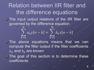
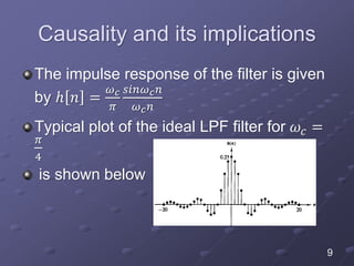
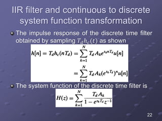
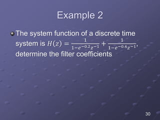
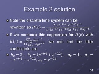
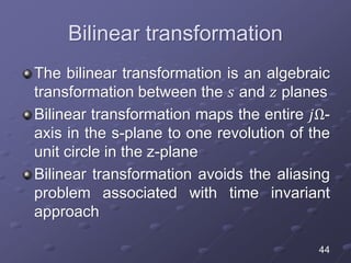
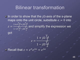
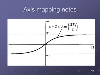
10. Causality and its implications
From the plot of ℎ[𝑛] it is clear that ℎ 𝑛 ≠
0 for 𝑛 < 0 which means that the filter is
not causal
If the filter is not causal this means that the
filter output samples 𝑦[𝑛] depends on the
future values of the input 𝑥[𝑛 + 1], 𝑥[𝑛 +
2] which is impossible to estimate
10

11. Processing continuous time
signal with digital filter
Consider a discrete-time filter is to be used
to low pass filter a continuous time signal
The complete system may be presented
as shown below
11

12. Determining specifications for a
discrete time filter
When designing a LPF we need its
magnitude frequency response to be as
shown
12

13. Design of discrete time IIR filters
from continuous time filters
The traditional approach to design IIR
filters involves the transformation of a
continuous-time filter into a discrete-time
filter meeting prescribed specifications
This design procedure can be achieved by
finding the system function 𝐻𝑐(𝑠) or the
impulse response of the continuous filter
ℎ 𝑐(𝑡)
13

14. Design of discrete time IIR filters
from continuous time filters
There are four well known analog filters
used in the design of IIR digital filters
these are
 Butterworth
 Chebyshev I
 Chebyshev II
 Elliptic
14

15. Design of discrete time IIR filters
from continuous time filters
The system function 𝐻(𝑧) or the impulse
response ℎ 𝑛 for the discrete-time filter is
obtained by using either
 Impulse invariance method
 Bilinear transformation
15

16. IIR filter design by Impulse
invariance
In the impulse invariance method we can
design an IIR filter by sampling the
impulse response of analog filter
according to
ℎ 𝑛 = 𝑇𝑑ℎ 𝑐 𝑛𝑇𝑑
Where 𝑇𝑑 represents the sampling interval
16

17. IIR filter design by Impulse
invariance
If the continuous time filter is band limited,
so that
𝐻𝑐 𝑗Ω = 0 Ω ≥
𝜋
𝑇𝑑
𝐻 𝑒 𝑗𝜔
= 𝐻𝑐(𝑗
𝜔
𝑇𝑑
) 𝜔 ≤ 𝜋
17

18. IIR filter design by Impulse
invariance
The discrete-time filter and the continuous
time filter frequency responses are related
by a linear scaling of the frequency axis
which is given by 𝜔 = Ω𝑇𝑑 for 𝜔 ≤ 𝜋
Where 𝜔 is the discrete frequency axis
and Ω is the continuous frequency axis
18

19. Practical IIR filter and aliasing
Any practical continuous filter can not be
exactly band limited
This means that the sampling process will
cause interference between successive
samples which causes aliasing as shown
19

20. Practical IIR filter and aliasing
The aliasing problem makes the impulse
invariance method not a suitable method for
the design of high pass filters
However if the continuous time filter
approaches zero at high frequencies, the
aliasing is negligible and can be ignored
20

21. IIR filter and continuous to discrete
system function transformation
Consider the system function of the
continuous-time filter expressed in terms of
partial fractions as shown below
The corresponding impulse response is
(inverse Laplace transform)
𝑁 represents the number
of poles
21

22. IIR filter and continuous to discrete
system function transformation
The impulse response of the discrete time filter
obtained by sampling 𝑇𝑑ℎ 𝑐(𝑡) as shown
The system function of the discrete time filter is
22

23. IIR filter and continuous to discrete
system function transformation
If we compare the system function for both
continuous time 𝐻𝑐 𝑠 and discrete time 𝐻(𝑧)
system function, we observe that a pole at
𝑠 = 𝑠 𝑘 in the S- plane transforms to a pole at
𝑧 = 𝑒 𝑠 𝑘 𝑇 𝑑 in the z plane
Also the coefficients in the partial fraction for
both 𝐻𝑐 𝑠 and 𝐻(𝑧) are equal, except for the
scaling multiplier 𝑇𝑑
23

24. IIR filter and continuous to discrete
system function transformation
Note that 𝑠 𝑘 is acomplex number which can be
written as 𝑠 𝑘 = 𝜎 + 𝑗𝜔 this means that 𝑧 =
𝑒 𝜎𝑇 𝑑 𝑒 𝑗𝜔𝑇 𝑑
If the real par of 𝑠 𝑘 is less than zero (𝜎 negative),
then 𝑧 < 1 , the corresponding pole in the
discrete time filter falls inside the unit circle
This means that the causal discrete time filter is
stable
24

25. Example 1
Example 1 convert the analog filter defined
by the system function 𝐻 𝑎 𝑠 =
1
(𝑠+0.1)2+9
into
a digital IIR filter by means of impulse
invariance method
25

26. Example1 solution
Solution
Since the filter system function 𝐻𝑐 𝑠 for the
continuous filter is given we can find
𝐻(𝑧) directly through the partial fraction (no
need to go back to the time domain and then
use sampling)
From 𝐻𝑐 𝑠 we can find that the filter has two
poles located at
𝑠1 = −0.1 + 𝑗3 and 𝑠2 = −0.1 − 𝑗3
26

27. Example1 solution
Solution
If we analyze 𝐻𝑐 𝑠 by the partial fraction
we get
To find 𝐻(𝑧) we use the expression
developed in slide 23
27

28. Example1 solution
If we plot the poles and zeros of the
previous example we can see that 𝜎 < 0
and both poles are located in the left side
of the s plane as shown below
28

29. Example 1 solution
If we manipulate 𝐻(𝑧) expression we find that
𝐻(𝑧) can be written as
If we compare this expression for 𝐻(𝑧) with
𝐻 𝑧 = 𝑘=0
𝑀
𝑏 𝑘 𝑧−𝑘
1+ 𝑘=1
𝑁
𝑎 𝑘 𝑧−𝑘 we can find the filter
coefficients are
𝑏0 = 1, 𝑏1 = −𝑒−0.1𝑇 𝑑cos(3𝑇𝑑), 𝑎0 = 1, 𝑎1 =
− 2𝑒−0.1𝑇 𝑑 cos 3𝑇𝑑 , 𝑎2 = 𝑒−0.2𝑇 𝑑,
29
2

30. Example 2
The system function of a discrete time
system is 𝐻 𝑧 =
1
1−𝑒−0.2 𝑧−1 +
1
1−𝑒−0.4 𝑧−1,
determine the filter coefficients
30

31. Example 2 solution
Note the discrete time system can be
rewritten as 𝐻 𝑧 =
2− 𝑒−0.4+𝑒−0.2 𝑧−1
1− 𝑒−0.4+𝑒−0.2 𝑧−1+𝑒−0.6 𝑧−2
If we compare this expression for 𝐻(𝑧) with
𝐻 𝑧 = 𝑘=0
𝑀
𝑏 𝑘 𝑧−𝑘
1+ 𝑘=1
𝑁
𝑎 𝑘 𝑧−𝑘 we can find the filter
coefficients are
𝑏0 = 2 , 𝑏1 = 𝑒−0.4
+ 𝑒−0.2
, 𝑎0 = 1 , 𝑎1 =
− 𝑒−0.4
− 𝑒−0.2
, 𝑎2 = 𝑒−0.6
31

32. Example 3
Design a Butterworth filter whose continuous
frequency response is given by
𝐻𝑐(𝑗Ω) 2 =
1
1+
Ω
Ω 𝑐
2𝑁
using the impulse invariance method
The filter specifications are
32

33. Example 3 solution
Solution
Since the parameter 𝑇𝑑 cancels in the impulse
invariance procedure we can select 𝑇𝑑 = 1 ,
therefore Ω = 𝜔
In order to deign the filter we need to transform
the discrete filter specifications to specifications
on the continuous time filter
33

34. Example 3 solution
Solution
The continuous time filter specifications became
The filter magnitude at the pass band and stop
band frequencies is given by
34

35. Example 3 solution
Solution
From the above magnitude conditions, the
magnitude squared of the continuous filter at
both the pass and stop bands is given by
0.89125 2 =
1
1+
0.2𝜋
Ω 𝑐
2𝑁
0.17783 2
=
1
1+
0.3𝜋
Ω 𝑐
2𝑁
35

36. Example 3 solution
Solution
If we solve the above two equations for 𝑁 and
Ω 𝑐 we got 𝑁 = 5.8858 ≈ 6 and Ω 𝑐 = 0.7032
Since 𝑁 = 6 then the filter has 12 poles of the
magnitude squared function 𝐻𝑐 𝑠 𝐻𝑐 −𝑠 =
1
1+
𝑆
Ω 𝑐
2𝑁
The poles can easily be found by using the
following matlab commands
36

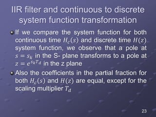
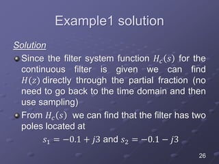
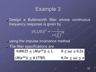
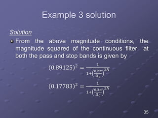
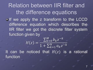
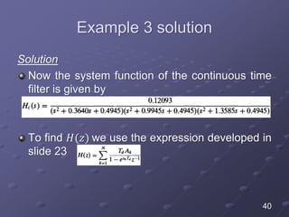
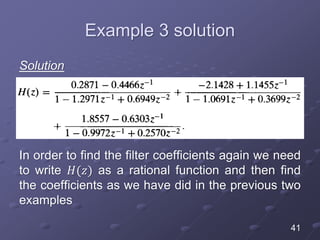
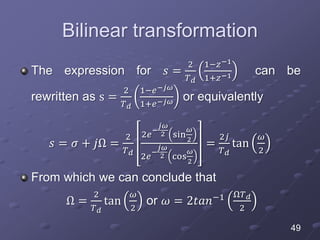
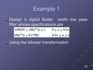
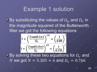
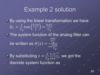
37. Example 3 solution
𝑎 = 1
b=[68.399 0 0 0 0 0 0 0 0 0 0 0 1]
[𝑧 𝑝 𝑘] = 𝑡𝑓2𝑧𝑝(𝑎, 𝑏)
37

38. Example 3 solution
Solution
The poles are uniformly
distributed in angle of
360°
12
= 30° on a circle of
radius Ω 𝑐 = 0.7032 as
shown
38

39. Example 3 solution
Solution
The poles that describe a stable system are
those poles located in the left side of the s-plane
The number of these poles is 6 and one solution
for these poles is on the assumption that the first
pole located a at an angle of 105°
39

40. Example 3 solution
Solution
Now the system function of the continuous time
filter is given by
To find 𝐻(𝑧) we use the expression developed in
slide 23
40

41. Example 3 solution
Solution
In order to find the filter coefficients again we need
to write 𝐻(𝑧) as a rational function and then find
the coefficients as we have did in the previous two
examples
41

42. Impulse invariance summery
To summarize, the impulse invariance method maps
the s-plane to the z-plane by sampling the impulse
response of continuous (analog) time filter
Impulse invariance suffers from aliasing problem
and therefore is not suitable for HPF design
42

43. Impulse invariance summery
In order to find the filter coefficients follow these steps
1. find 𝐻𝑐 𝑠 , expand it in partial fraction, find the poles
of 𝐻𝑐 𝑠
2. Next find the discrete system function according to
𝐻 𝑧 = 𝑘=1
𝑁 𝑇 𝑑 𝐴 𝑘
1−𝑒 𝑠 𝑘 𝑇 𝑑 𝑧−1
3. Convert 𝐻(𝑧) to rational function
4. Compare the rational expression for 𝐻(𝑧) with
𝐻 𝑧 = 𝑘=0
𝑀
𝑏 𝑘 𝑧−𝑘
1+ 𝑘=1
𝑁 𝑎 𝑘 𝑧−𝑘 and determine the coefficients
accordingly
43

44. Bilinear transformation
The bilinear transformation is an algebraic
transformation between the 𝑠 and 𝑧 planes
Bilinear transformation maps the entire 𝑗Ω-
axis in the s-plane to one revolution of the
unit circle in the z-plane
Bilinear transformation avoids the aliasing
problem associated with time invariant
approach
44

45. Bilinear transformation
The bilinear transformation corresponds to
replacing 𝑠 by
𝑠 =
2
𝑇𝑑
1 − 𝑧−1
1 + 𝑧−1
This means that the discrete and
continuous system functions are related by
𝐻 𝑧 = 𝐻𝑐
2
𝑇𝑑
1 − 𝑧−1
1 + 𝑧−1
45

46. Bilinear transformation
To develop the properties of the algebraic
transformation we solve for 𝑧 to obtain
𝑧 =
2
𝑇𝑑
1 +
𝑇𝑑
2
𝑠
1 −
𝑇𝑑
2
𝑠
Substituting 𝑠 = 𝜎 + 𝑗𝜔, we got
𝑧 =
1 + 𝜎
𝑇𝑑
2
+ 𝑗Ω
𝑇𝑑
2
1 − 𝜎
𝑇𝑑
2
− 𝑗Ω
𝑇𝑑
2
46

47. Bilinear transformation
Again as in the time invariant procedure, if 𝜎 <
0, 𝑧 < 1, for any value of Ω
This means the poles fall in the left half of the s-
plane or inside the unit circle of the z-plane,
which means that the system is stable
Similarly if of 𝜎 > 0, 𝑧 > 1, for any value of Ω
The poles fall in the right half of the s-plane or
outside the unit circle of the z-plane, which
means that the system is unstable
47

48. Bilinear transformation
In order to show that the 𝑗Ω-axis of the s-plane
maps onto the unit circle, substitute 𝜎 = 0 into
𝑧 =
1+𝜎
𝑇 𝑑
2
+𝑗Ω
𝑇 𝑑
2
1−𝜎
𝑇 𝑑
2
−𝑗Ω
𝑇 𝑑
2
and simplify the expression we
got
𝑧 =
1 + 𝑗Ω
𝑇𝑑
2
1 − 𝑗Ω
𝑇𝑑
2
Recall that 𝑧 = 𝑒 𝜎 𝑒 𝑗𝜔 = 𝑒 𝑗𝜔
48

49. Bilinear transformation
The expression for 𝑠 =
2
𝑇 𝑑
1−𝑧−1
1+𝑧−1 can be
rewritten as s =
2
𝑇 𝑑
1−𝑒−𝑗𝜔
1+𝑒−𝑗𝜔 or equivalently
𝑠 = 𝜎 + 𝑗Ω =
2
𝑇 𝑑
2𝑒
−
𝑗𝜔
2 sin
𝜔
2
2𝑒
−
𝑗𝜔
2 cos
𝜔
2
=
2𝑗
𝑇 𝑑
tan
𝜔
2
From which we can conclude that
Ω =
2
𝑇 𝑑
tan
𝜔
2
or 𝜔 = 2𝑡𝑎𝑛−1 Ω𝑇 𝑑
2
49

50. Mapping between the z-plane
and the s-plane
The properties of the bilinear transformation as
mapping from the s-plane to the z-plane are
illustrated graphically as shown below
50

51. Axis mapping notes
Note that the Bilinear transformation maps
the range of continuous frequencies 0 ≤
Ω ≤ ∞ maps to 0 ≤ 𝜔 ≤ 𝜋 on the discrete
frequency axis
Also the range of continuous frequencies
− ∞ ≤ Ω ≤ 0 maps to −𝜋 ≤ 𝜔 ≤ 0 on the
discrete frequency axis as illustrated in the
next slide
51

52. Axis mapping notes
52

53. Example 1
Design a digital Butter worth low pass
filter whose specifications are
Using the bilinear transformation
53

54. Example 1 solution
The design procedure starts by reflecting the
specifications of the discrete filter to
specifications of the digital filter as shown
Let 𝑇𝑑 = 1
54

55. Example 1 solution
The magnitude of the filter at the pass
band frequency Ω 𝑝 = 2 tan
0.2𝜋
2
is given
by
Also note that the magnitude of the filter at
the stop band Ω 𝑠 = 2 tan
0.3𝜋
2
is given by
55

56. Example 1 solution
By substituting the values of Ω 𝑝 and Ω 𝑠 in
the magnitude squared of the Butterworth
filter we got the following equations
By solving these two equations for Ω 𝑐 and
𝑁 we got 𝑁 = 5.305 ≈ 6 and Ω 𝑐 = 0.766
56

57. Example 1 solution
If we plot the poles of 𝐻𝑐 𝑠 2
of the filter
we got the following graph
57

58. Example 1 solution
From the pole plot it can be shown that
58

59. Example 2
Design a single pole low pass digital filter
with a 3-dB bandwidth of 0.2𝜋, using the
bilinear transformation applied to the
analog filter defined by 𝐻 𝑠 =
Ω 𝑐
𝑠+Ω 𝑐
where
Ω 𝑐 is the 3-dB bandwidth of the filter
59

60. Example 2 solution
By using the linear transformation we have
Ω 𝑐 =
2
𝑇 𝑑
tan
0.2𝜋
2
=
0.65
𝑇 𝑑
The system function of the analog filter can
be written as 𝐻 𝑠 =
0.65
𝑇 𝑑
𝑠+
0.65
𝑇 𝑑
By substituting 𝑠 =
2
𝑇 𝑑
1−𝑧−1
1+𝑧−1, we got the
discrete system function as
60

61. Example 2 solution
𝐻 𝑧 =
0.65
𝑇 𝑑
2
1−𝑧−1
1+𝑧−1+
0.65
𝑇 𝑑
= 0.245
1+𝑧−1
1−0.509𝑧−1
61

62. IIR filter design in MATALB
We have seen from the previous discussion both
the impulse invariance and bilinear
transformations needs too many computations
A simpler way to design an IIR filter can be done
easily with the aid of MATLAB
It is easy to show this by an example
62

63. IIR filter design in MATLAB
Design a band pass filter with the following
specifications
 Pass band frequencies from 1000 to 2000 Hz
 The stop bands starting 500 Hz away on either side
 A 10 kHz sampling frequency
 At most 1 dB of pass band ripple and at least 60 dB of
stop band attenuation
63

64. IIR filter design in MATLAB
Solution
 In order to design the filter we need to specify its
coefficients
 This can be achieved by using the following
statements in MATLAB
 𝑓𝑠 = 10 𝑘𝐻𝑧 % Sampling frequency
 𝑓𝑝1 = 1 𝑘𝐻𝑧 % The first band pass frequency
 𝑓𝑝2 = 2 𝑘𝐻𝑧 % The second band pass frequency
 𝑓𝑠1 = 500 𝐻𝑧 % The first stop band frequency
 𝑓𝑠2 = 2500 𝐻𝑧 % The second stop band frequency
64

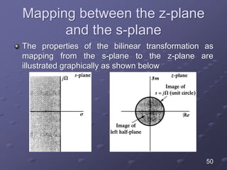
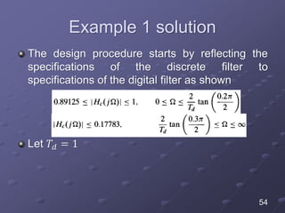
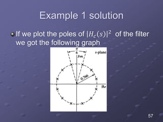
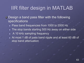
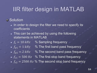
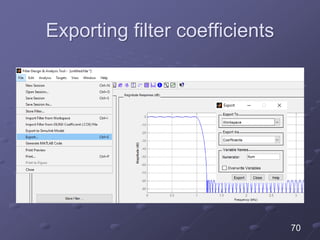
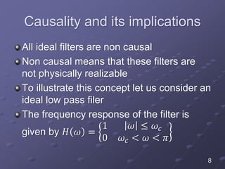
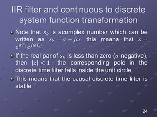
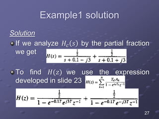
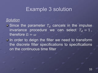
65. IIR filter design in MATLAB
 𝑅𝑝 = 1 𝑑𝐵 % The ripple in the pass band
 𝑅 𝑆 = 60 𝑑𝐵 % The attenuation in the stop band
 The filter order and normalized frequencies can be
computed by using the following statement
 [𝑛, 𝑊𝑛] = 𝑏𝑢𝑡𝑡𝑜𝑟𝑑
𝑓𝑝1 𝑓𝑝2
𝑓𝑠
,
𝑓𝑠1 𝑓𝑠2
𝑓𝑠
, 𝑅 𝑝, 𝑅 𝑠
 The filter coefficients can be computed from the
following statements
 𝑏, 𝑎 = 𝑏𝑢𝑡𝑡𝑒𝑟 𝑛, 𝑊𝑛 ;
65

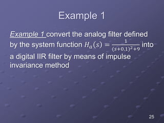
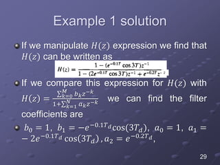
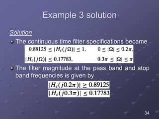
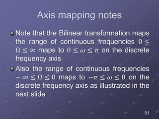
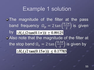
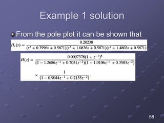
66. IIR filter design in MATLAB
More examples to design IIR filter is by the use of these
statements
 [𝑏, 𝑎] = 𝑏𝑢𝑡𝑡𝑒𝑟(𝑛, 𝑊𝑛, 𝑜𝑝𝑡𝑖𝑜𝑛𝑠)
 [𝑏, 𝑎] = 𝑏𝑢𝑡𝑡𝑒𝑟(5,0.4); % Lowpass Butterworth
 [𝑏, 𝑎] = 𝑐ℎ𝑒𝑏𝑦1(𝑛, 𝑅𝑝, 𝑊𝑛, 𝑜𝑝𝑡𝑖𝑜𝑛𝑠)
 [𝑏, 𝑎] = 𝑐ℎ𝑒𝑏𝑦1(4,1, [0.4 0.7]); % Bandpass Chebyshev Type I
 [𝑏, 𝑎] = 𝑐ℎ𝑒𝑏𝑦2(𝑛, 𝑅𝑠, 𝑊𝑛, 𝑜𝑝𝑡𝑖𝑜𝑛𝑠)
 [𝑏, 𝑎] = 𝑐ℎ𝑒𝑏𝑦2(6,60,0.8, ′ℎ𝑖𝑔ℎ′); % Highpass Chebyshev Type II
 [𝑏, 𝑎] = 𝑒𝑙𝑙𝑖𝑝(𝑛, 𝑅𝑝, 𝑅𝑠, 𝑊𝑛, 𝑜𝑝𝑡𝑖𝑜𝑛𝑠)
 [𝑏, 𝑎] = 𝑒𝑙𝑙𝑖𝑝(3,1,60, [0.4 0.7], ′𝑠𝑡𝑜𝑝′); % Bandstop elliptic
66

67. Filter design in MATLAB
We can design IIR or FIR filters in MATALB
using the filter design and analysis tool
FDATOOL
In the command window of MATLAB type
FDATOOL
A window the filter design window will appear as
shown in the next slide
67

68. 68

69. Using FDATOOL
To design a filter, you need to specify the
sampling rate, pass and stop band frequencies
You can also determine the filter type,
implementation, FIR or IIR
Once the filter is designed you can view or
export the filter coefficients to workspace or file
using the command file as illustrated in the next
slide
69

70. Exporting filter coefficients
70