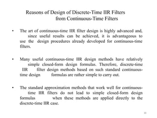
The document discusses the Discrete Fourier Transform (DFT) and its computational complexity, outlining how each DFT coefficient requires significant real operations and introducing fast methods like the Fast Fourier Transform (FFT) that leverage symmetry and periodicity. It also covers filter design techniques for digital systems, specifically focusing on Infinite Impulse Response (IIR) filters, including their specifications, implementation, and common types like Butterworth and Chebyshev filters. Overall, it presents principles and complexities around DFT computation, as well as practical considerations in the design of digital filters.

1. Discrete Fourier Transform
1
• The DFT pair was given
as N  1 1
N
N  1
 
j 2  / N
kn
X k 
 n 
0
 x[n]e
 j 2  / N kn x[n]  
k  0 X k
e
• Baseline for computational
complexity:
– Each DFT coefficient requires
• N complex multiplications
• N-1 complex additions
– All N DFT coefficients require
• N2 complex multiplications
• N(N-1) complex additions
• Complexity in terms of real operations
• 4N2 real multiplications
• 2N(N-1) real additions
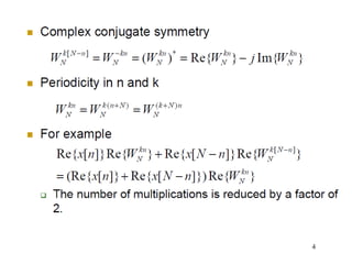
• Most fast methods are based on symmetry
properties
– Conjugate symmetry
– Periodicity in n and k
e  j2  / N k N  n 
 e  j2  / N kN
e  j2  / N k  n   e j2  / N kn
e  j2  / N kn
 e  j2  / N k n  N 
 e j2  / N k  N n

2. Direct computation of DFT
2

3. Direct computation of DFT
3

4. 4

5. FFT
5

6. 6
2
rk
N
N
rk
N / 2
N
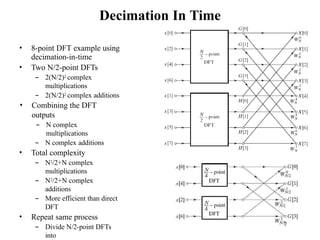
Decimation-In-Time FFT Algorithms
• Makes use of both symmetry and periodicity
• Consider special case of N an integer power of
2
• Separate x[n] into two sequence of length N/2
– Even indexed samples in the first sequence
– Odd indexed samples in the other sequence
X k
 
N  1
 x[n]e
n  0
 j2  / N kn
N  1

x[n
]e
n
even

 j2  / N kn
N  1
 x[n]e
n odd

 j 2  / N kn
• Substitute variables n=2r for n even and n=2r+1 for
odd N / 2  1
X k
 

r  0
x[2
r ]W
 1]W
2 r  1 k
N / 2  1
 
x[2 r
r  0
N / 2
 1
N / 2  1
 
r  0
x[2
r ]W
N
r  0
N / 2
 W k
 x[2 r  1]W rk
k
 G k   W H k

• G[k] and H[k] are the N/2-point DFT’s of each
subsequence

7. Decimation In Time
• 8-point DFT example using
decimation-in-time
• Two N/2-point DFTs
– 2(N/2)2 complex
multiplications
– 2(N/2)2 complex additions
• Combining the DFT
outputs
– N complex
multiplications
– N complex additions
• Total complexity
– N2/2+N complex
multiplications
– N2/2+N complex
additions
– More efficient than direct
DFT
• Repeat same process
– Divide N/2-point DFTs
into
7

8. Decimation In Time Cont’d
• After two steps of decimation in
time
• Repeat until we’re left with two-point
DFT’s
8

9. Decimation-In-Time FFT Algorithm
• Final flow graph for 8-point decimation in
time
• Complexity:
– Nlog2N complex multiplications and
additions
9

10. Butterfly Computation
• Flow graph constitutes of
butterflies
• We can implement each butterfly with one multiplication
• Final complexity for decimation-in-time FFT
– (N/2)log2N complex multiplications and
additions
10

11. 11
In-Place Computation
• Decimation-in-time flow graphs require two sets of
registers
– Input and output for each stage
• Note the arrangement of the input indices
– Bit reversed indexing
X 0 0

 x 0

 X 0 000  x
000

X 0 1

 x 4

 X 0 001  x
100

X 0 2

 x 2

 X 0 010  x
010

X 0 3

 x 6

 X 0 011  x
110

X 0 4

 x 1

 X 0 100  x
001

X 0 5

 x 5

 X 0 101  x
101


12. 12
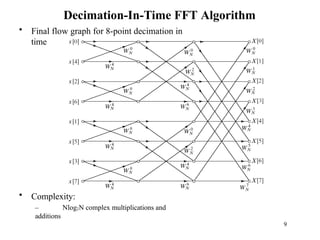
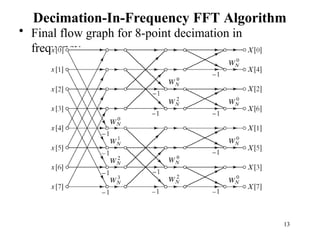
Decimation-In-Frequency FFT Algorithm
nk
N
N N N
n 2
r
N
N N / 2
N / 2
X k
 
• The DFT equation
N  1

n  0
• Split the DFT equation into even and odd frequency
indexes
N  1 N / 2  1 N  1
x[n]W
X 2 r
 
 x[n]W n 2 r

x[n]W n 2 r 


n  0
x[n]W n 2 r
n  0
• Substitute variables to get
n  N / 2
N / 2  1 N / 2  1
  x[n
n  0
N / 2  1
X 2 r
 

n 
0
x[n]W  N / 2 ]W
n  N / 2 2 r  
n 
0
x[n]  x[n  N / 2 ]W nr
• Similarly for odd-numbered frequencies
N / 2  1
X 2 r  1    x[n]  x[n
 N / 2 ]W n 2 r  1 
n 
0

13. Decimation-In-Frequency FFT Algorithm
• Final flow graph for 8-point decimation in
frequency
13

14. x n  y n

D/C
H(ej)
C/D
He j   H j / T 
c
Filter Design Techniques
• Any discrete-time system that modifies certain frequencies
• Frequency-selective filters pass only certain frequencies
• Filter Design Steps
– Specification
• Problem or application specific
– Approximation of specification with a discrete-time system
• Our focus is to go from spec to discrete-time system
– Implementation
• Realization of discrete-time systems depends on target technology
• We already studied the use of discrete-time systems to implement a
continuous-time system
– If our specifications are given in continuous time we can use
xc(t)
yr(t)
 

14
IIR Filters

15. Digital Filter Specifications
• Only the magnitude approximation problem
• Four basic types of ideal filters with magnitude
responses as shown below (Piecewise flat)
15

16. Digital Filter Specifications
16
• These filters are unealisable because (one of the
following is sufficient)
– their impulse responses infinitely long non-
causal
– Their amplitude responses cannot be equal to
a constant over a band of frequencies
Another perspective that provides some
understanding can be obtained by looking at
the ideal amplitude squared.

17. Digital Filter Specifications
17
• The realisable squared amplitude response
transfer function (and its differential) is
continuous in
• Such functions 
– if IIR can be infinite at point but around
that point cannot be zero.
– if FIR cannot be infinite anywhere.
• Hence previous differential of ideal response
is unrealisable

18. Digital Filter Specifications
• For example the magnitude response of a
digital lowpass filter may be given as indicated
below
18

19. p
• In the passband 0     we
requireG ( e j ) 
1
that with a deviation
 p
p
1    G ( e j )  1   p ,   
p
  

• In the stopband  s we re qs
uire G ( e
j
)  0
that with a deviation
G ( e j )   s ,  s   

Digital Filter Specifications
19

20. p
Filter specification parameters


s

p

s
• - passband edge frequency
• - stopband edge frequency
• - peak ripple value in the
passband
• - peak ripple value in the
stopband
Digital Filter Specifications
20

21. • Practical specifications are often given
in terms of loss function (in dB)
• G ( )

 20 log 10 G ( e
j )
• Peak passband
ripple p   20 log
 10 (1   p ) dB
• Minimum stopband attenuation
 s   20
log 10 ( s ) dB
Digital Filter Specifications
21

22. p
s
p
• In practice, passband edge frequency F
and
stopband edge frequency arFes
specified in Hz
• For digital filter design, normalized
bandedge frequencies need to be computed
from
specifications in Hz using  2
F
p
 
 FT
p
FT
p
 2 FT
2
Fs

s
 s
   2 F
T
FT FT
250
Digital Filter Specifications

23. p s
T
 7
• Example - Let F
kHz,
F  3
F  25 kHz
kHz,
and
• Then

2( 7  10 3 )
p  3  0 .56

25  10
2( 3  10 3 )
 s  3  0 .24

25  10
Digital Filter Specifications
23

24. IIR Digital Filter Design
24
Standard approach
(1)Convert the digital filter specifications into
an analogue prototype lowpass filter
specifications
(2)Determine the analogue lowpass filter
transfer function H a ( s )
(3)Transform H a ( s ) by replacing the
complex variable to the digital transfer
function
G ( z )

25. IIR Digital Filter Design
25
• This approach has been widely used for
the following reasons:
(1)Analogue approximation techniques
are highly advanced
(2)They usually yield closed-
form solutions
(3)Extensive tables are available
for analogue filter design
(4)Very often applications require
digital simulation of analogue systems

26. D a ( s )
• Let an analogue transfer function
be H ( s )

a
Pa
( s )
where the subscript “a” indicates
the analogue domain
• A digital transfer function derived from
this is denoted as
G ( z )

P
( z )
D
( z )
IIR Digital Filter Design
26

27. IIR Digital Filter Design
27
• Basic idea behind the conversion of H ( s ) intoG
( z )
a
is to apply a mapping from the s-
domain to the z-
domain so that essential properties of the
analogue frequency response are preserved
• Thus mapping function should be such that
– Imaginary (j  ) axis in the s-plane
be mapped onto the unit circle of the
z-plane
– A stable analogue transfer function be
mapped into a stable digital transfer function

28. Specification for effective frequency response of a continuous-time
lowpass filter and its corresponding specifications for discrete-time
system.
dp or d1 passband ripple
ds or d2 stopband ripple
Wp, wp passband edge frequency
Ws, ws stopband edge frequency
e2 passband ripple parameter
1 – dp = 1/1 + e2
BW bandwidth = wu – wl
wc 3-dB cutoff frequency
wu, wl upper and lower 3-dB cutoff
frequensies
Dw transition band = |wp – ws|
Ap passband ripple in dB
=  20log10(1 
dp) As stopband attenuation in
dB
= -
20log10(ds) 28

29. 29
Design of Discrete-Time IIR Filters
• From Analog (Continuous-Time)
Filters
– Approximation of Derivatives
– Impulse Invariance
– the Bilinear Transformation

30. Reasons of Design of Discrete-Time IIR Filters
from Continuous-Time Filters
30
• The art of continuous-time IIR filter design is highly advanced and,
since useful results can be achieved, it is advantageous to
use the design procedures already developed for continuous-time
filters.
• Many useful continuous-time IIR design methods have relatively
simple closed-form design formulas. Therefore, discrete-time
IIR filter design methods based on such standard continuous-
time design formulas are rather simple to carry out.
• The standard approximation methods that work well for continuous-
time IIR filters do not lead to simple closed-form design
formulas when these methods are applied directly to the
discrete-time IIR case.

31. 31
Characteristics of Commonly Used Analog Filters
• Butterworth Filter
• Chebyshev Filter
– Chebyshev Type I
– Chebyshev Type II of Inverse Chebyshev Filter

32. 32
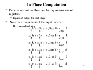
Butterworth Filter
• Lowpass Butterworth filters are all-pole filters characterized by the magnitude-squared
frequency response
|H(W)|2 = 1/[1 + (W/Wc)2N] = 1/[1 + e2(W/Wp)2N]
where N is the order of the filter, Wc is its – 3-dB frequency (cutoff frequency), Wp
is the bandpass edge frequency, and 1/(1 + e2) is the band-edge value of |
H(W)|2.
• At W = Ws (where Ws is the stopband edge frequency) we have
1/[1 + e2(Ws/Wp)2N] = d2
2
and
N = (1/2)log10[(1/d2
2) – 1]/log10(Ws/Wc) = log10(d/e)/log10(Ws/Wp)
where d2= 1/1 + d2
2.
• Thus the Butterworth filter is completely characterized by the parameters N, d2, e, and
the ratio Ws/Wp.

33. 2
H j  c
Butterworth Lowpass
Filters
• Passband is designed to be maximally flat
• The magnitude-squared function is of the
form 
1
c
1  j / j
2 N
H s 
2

1  s / j
1
c
2 N
sk
  1 1 / 2 N
j    e
 j / 2 N 2 k  N  1 
c c
for k  0,1,...,2N - 1
c
33

34. Frequency response of lowpass Butterworth
filters
34

35. 35
Chebyshev Filters
• The magnitude squared response of the analog lowpass Type I
Chebyshev filter of Nth order is given by:
|H(W)|2 = 1/[1 + e2T 2(W/W )].
N
where TN(W) is the Chebyshev polynomial of order
N: TN(W) = cos(Ncos-1 W), |W|  1,
= cosh(Ncosh-1 W), |W| >
1.
The polynomial can be derived via a recurrence relation given
by Tr(W) = 2WTr-1(W) – Tr-2(W), r  2,
with T0(W) = 1 and T1(W) = W.
• The magnitude squared response of the analog lowpass Type II or
inverse Chebyshev filter of Nth order is given by:
|H(W)|2 = 1/[1 + e2{TN(Ws/Wp)/ TN(Ws/W)}2].

36. c
N
N
c
Chebyshev
Filters
• Equiripple in the passband and monotonic in the stopband
• Or equiripple in the stopband and monotonic in the
passband
2 1

H  j 
1   2
V 2
 /  
V x   cos N cos  1 x 
36

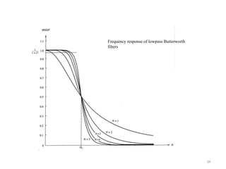
37. N
Frequency response of
lowpass Type I Chebyshev
filter
|H(W)|2 = 1/[1 + e2T 2(W/W )]
Frequency response of
lowpass Type II Chebyshev filter
|H(W)|2 = 1/[1 + e2{T 2(W /W )/T 2(W /W)}]
N
s
p
N
s
37

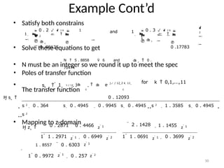
38. 38
N = log10[( 1 - d 2 +  1 – d 2(1 + e2))/ed
]/log 2 2 2
10
[(W /W ) +  (W /W )2 –
1 ]
s p s p
= [cosh-1(d/e)]/[cosh-1(Ws/Wp)]
for both Type I and II Chebyshev filters, and
where d2 = 1/  1 + d2.
• The poles of a Type I Chebyshev filter lie on an ellipse in the s-plane with major
axis r1 = Wp{(b2 + 1)/2b] and minor axis r1 = Wp{(b2 - 1)/2b] where b is related to
e according to
b = {[ 1 + e2 + 1]/e}1/N
• The zeros of a Type II Chebyshev filter are located on the imaginary axis.

39. Type I: pole positions are
xk = r2cosfk
yk = r1sinfk
fk = [p/2] + [(2k + 1)p/2N]
r1 = Wp[b2 + 1]/2b
r2 = Wp[b2 – 1]/2b
b = {[ 1 + e2 + 1]/e}1/N
Type II: zero positions are
sk = jWs/sinfk
and pole positions are
vk = Wsxk/ x 2 + y 2
k
k
wk = Wsyk/ x 2 + y 2
k
k 2
b = {[1 +  1 – d 2
]/d }1/N
Determination of the pole locations
for a Chebyshev filter.
k = 0, 1, …, N-1.
39

40. Approximation of Derivative Method
• Approximation of derivative method is the simplest one for converting an
analog filter into a digital filter by approximating the differential equation
by an equivalent difference equation.
– For the derivative dy(t)/dt at time t = nT, we substitute the backward difference
[y(nT) – y(nT – T)]/T. Thus

t  nT
 T )

y [ n ]  y [ n  1]
T
where T represents the sampling period. Then, s = (1 – z-1)/T
– The second derivative d2y(t)/dt2 is derived into second difference as follow:

t  nT T 2
y [ n ]  2 y [ n  1]  y [ n  2 ]
which s2 = [(1 – z-1)/T]2. So, for the kth derivative of y(t), sk = [(1 – z-1)/T]k.
dy ( t ) y ( nT )  y ( nT
dt T
dy
( t )
dt
40

41. Approximation of Derivative
Method
41
• Hence, the system function for the digital IIR filter obtained as a result of
the approximation of the derivatives by finite difference is
H(z) = Ha(s)|s=(z-1)/Tz
• It is clear that points in the LHP of the s-plane are mapped into the
corresponding points inside the unit circle in the z-plane and points in
the RHP of the s-plane are mapped into points outside this circle.
– Consequently, a stable analog filter is transformed into a stable digital filter due
to this mapping property.
jW
Unit circle
s
s-
plane
z-plane

42. Example: Approximation of derivative method
Convert the analog bandpass filter with system function
Ha(s) = 1/[(s + 0.1)2 + 9]
Into a digital IIR filter by use of the backward difference for the
derivative.
Substitute for s = (1 – z-1)/T into Ha(s) yields
H(z) = 1/[((1 – z-1)/T) + 0.1)2
+ 9]
H ( z ) 
T 2
1  0 .2 T  9 .01 T 2
 1
1 
2 ( 1  0 .1 T ) z
 1
z
 2
1  0 .2 T  9 .01 T 2
1  0 .2 T  9 .01 T 2
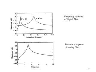
T can be selected to satisfied specification of designed filter. For example, if T =
0.1, the poles are located at
p1,2
= 0.91  j0.27 = 0.949exp[
j16.5o]
42

43. • If the continuous-time filter is bandlimited to
H c
 j   0
c 
Filter Design by Impulse Invariance
• Remember impulse invariance
– Mapping a continuous-time impulse response to discrete-time
– Mapping a continuous-time frequency response to discrete-time
hn  
T h
nT

d
c
d
   2

H e j
   H  j  j
c
k 

 Td
Td

k


j

 

   /
T d
H e   H 
j


Td

 

• If we start from discrete-time specifications Td cancels out
– Start with discrete-time spec in terms of 
– Go to continuous-time =  /T and design continuous-time
filter
– Use impulse invariance to map it back to discrete-time = T
• Works best for bandlimited filters due to possible aliasing
43

44. Impulse Invariance of System Functions
• Develop impulse invariance relation between system
functions
• Partial fraction expansion of transfer function
H s  

N
A k
c
• Corresponding impulse response

N
h t    
c k  1
k  1 s
 s k



A
e
s k t
0
t 
0
t  0
• Impulse response of discrete-time filter


 T dh c nT d 
 
h n
• System
function
N
s k nT d


N s k T d
n 

u n

u n   T d A k
e
k  1

k 
1
T d A k
e
 
H z
N T
A
d
k


k 
1
1  e
s k T d
z
 1
• Pole s=sk in s-domain transform into pole at e
s k T d
k
44

45. • Step 1: define specifications of filter
– Ripple in frequency bands
– Critical frequencies: passband edge, stopband edge, and/or cutoff frequencies.
– Filter band type: lowpass, highpass, bandpass, bandstop.
• Step 2: linear transform critical frequencies as follow
W = w/Td
• Step 3: select filter structure type and its order: Bessel, Butterworth,
Chebyshev type I, Chebyshev type II or inverse Chebyshev, elliptic.
• Step 4: convert Ha(s) to H(z) using linear transform in step 2.
• Step 5: verify the result. If it does not meet requirement, return to step 3.
Impulse Invariant Algorithm
45

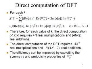
46. Example: Impulse invariant method
Convert the analog filter with system function
Ha(s) = [s + 0.1]/[(s + 0.1)2 + 9]
into a digital IIR filter by means of the impulse invariance method.
The analog filter has a zero at s = - 0.1 and a pair of complex conjugate poles at pk = - 0.1 
j3. Thus,
H s  
a
1 1
2
 2
s  0 .1  j 3 s  0 .1  j
3
Then
H  z  
1
 2
1  e
46
1
2
 0 .1 T
e
j 3 T
z
 1
1  e
 0 .1 T
e
 j 3 T
z
 1

47. Frequency response
of digital filter.
Frequency response
of analog filter.
47

48. Disadvantage of previous
techniques: frequency
warping  aliasing effect
and error in specifications
48
of designed filter (frequencies)
So, prewarping of frequency
is considered.



49. H j 
Example
• Impulse invariance applied to
Butterworth 0 . 89125  H e j   1 0    0 . 2

0 . 3   

H e j   0.17783
• Since sampling rate Td cancels out we can assume Td=1
• Map spec to continuous time
0 . 89125  H  j   1
H  j   0.17783
0    0 . 2

0 . 3    

• Butterworth filter is monotonic so spec will be satisfied if
H c
j0 .2    0 .89125 and H c
j0 .3    0.17783 2

1
c
1  j / j
c 
2
N
• Determine N and c to satisfy these conditions
49

50.  1 
Example Cont’d
• Satisfy both constrains

2


1     

and 1     








 0 . 3   2 N 
1
 c 
0 .89125
  c

0 .17783
• Solve these equations to get
 0 . 2   2 N  1
 2
N  5 . 8858  6 and  c
 0 .
70474
sk  
• N must be an integer so we round it up to meet the spec
• Poles of transfer function
• 1 / 12 j    e
 j / 12 2 k  11 
c c
for k  0,1,...,11
The transfer function
H s   0 . 12093
 0 . 9945 s  0 . 4945 s 2
 1 . 3585 s  0 . 4945 
s 2
 0 . 364 s  0 . 4945
s 2
• Mapping to z-domain
H z   0 . 2871  0 . 4466 z  1  2 . 1428  1 . 1455 z  1

z  1
50
1  1 . 2971  0 . 6949 z  2 1  1 . 0691 z  1  0 . 3699 z  2
1 . 8557  0 . 6303 z  1

z  1
1  0 . 9972  0 . 257 z  2

51. THANK
YOU