Decision Tree Learningis a widely used predictive model for supervised learning that
spans over a number of practical applications in various areas.
It is used for both classification and regression tasks.
The decision tree model basically represents logical rules that predict the value of a
target variable by inferring from data features.
The model performs an inductive inference that reaches a general conclusion from observed
examples.
This model is variably used for solving complex classification applications.
Decision tree is a concept tree which summarizes the information contained in the training
dataset in the form of a tree structure.
Once the concept model is built, test data can be easily classified.
3.
This model canbe used to classify both categorical target variables and continuous-valued target
variables.
Given a training dataset X, this model computes a hypothesis function f(X) as decision tree.
Inputs to the model are data instances or objects with a set of features or attributes which can be
discrete or continuous and the output of the model is a decision tree which predicts or classifies the
target class for the test data object.
In statistical terms, attributes or features are called as independent variables.
The target feature or target class is called as response variable which indicates the category we need
to predict on a test object.
The decision tree learning model generates a complete hypothesis space in the form of a tree
structure with the given training dataset and allows us to search through the possible set of
hypotheses which in fact would be a smaller decision tree as we walk through the tree. This kind of
search bias is called as preference bias.
4.
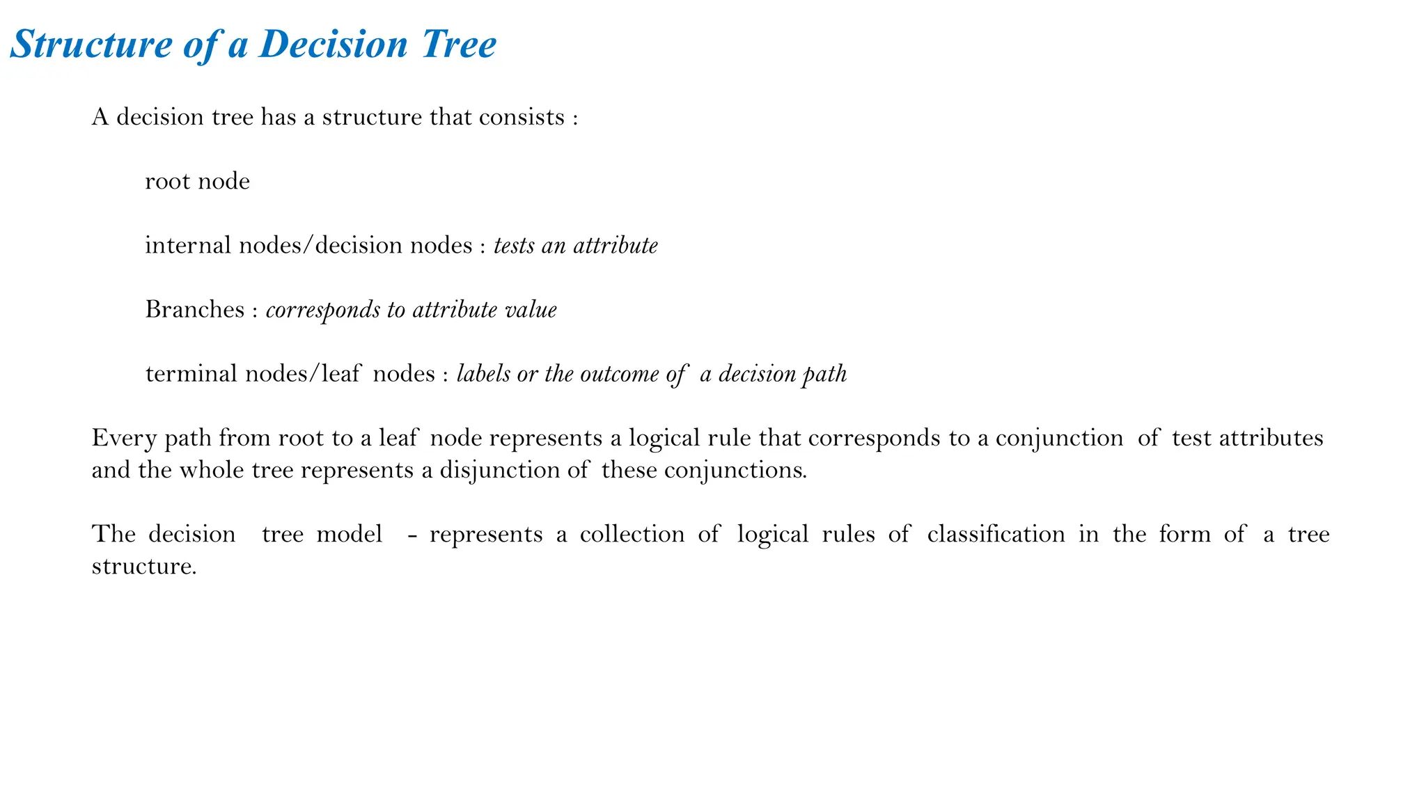
Structure of aDecision Tree
A decision tree has a structure that consists :
root node
internal nodes/decision nodes : tests an attribute
Branches : corresponds to attribute value
terminal nodes/leaf nodes : labels or the outcome of a decision path
Every path from root to a leaf node represents a logical rule that corresponds to a conjunction of test attributes
and the whole tree represents a disjunction of these conjunctions.
The decision tree model - represents a collection of logical rules of classification in the form of a tree
structure.
5.
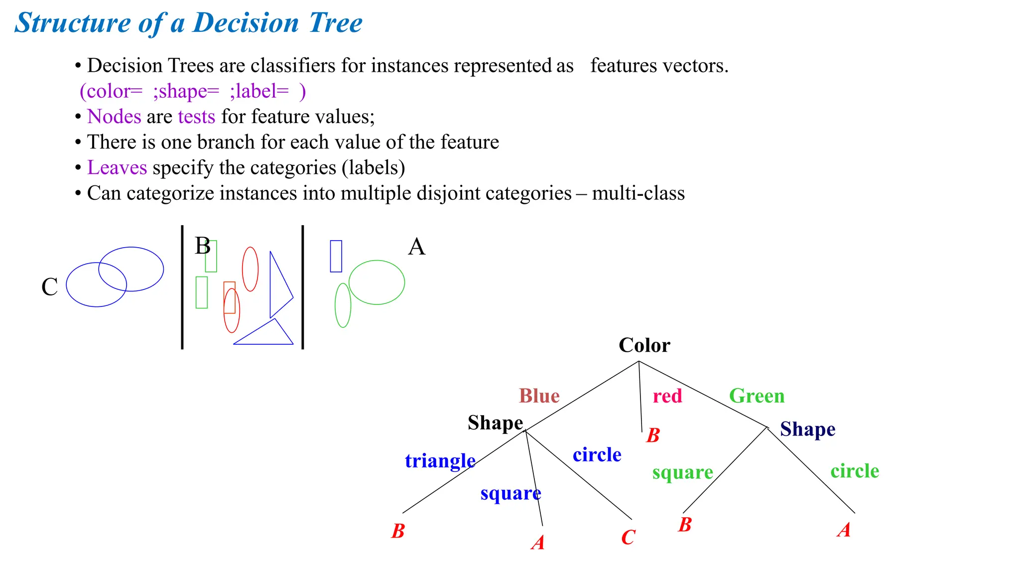
A
C
B
Structure of aDecision Tree
• Decision Trees are classifiers for instances represented as features vectors.
(color= ;shape= ;label= )
• Nodes are tests for feature values;
• There is one branch for each value of the feature
• Leaves specify the categories (labels)
• Can categorize instances into multiple disjoint categories – multi-class
Color
Shape
Blue red Green
Shape
square
triangle circle
circle
square
A
B
C
A
B
B
6.
A decision treeconsists of two major procedures
1. Building the Tree
Goal
Construct a decision tree with the given training dataset.
The tree is constructed in a top-down fashion.
It starts from the root node.
At every level of tree construction, we need to find the best split attribute or best decision node
among all attributes.
This process is recursive and continued until we end up in the last level of the tree or finding a leaf
node which cannot be split further.
The tree construction is complete when all the test conditions lead to a leaf node.
The leaf node contains the target class or output of classification.
Output
Decision tree representing the complete hypothesis space.
Structure of a Decision Tree
7.
2.Knowledge Inference orClassification
Goal
Given a test instance, infer to the target class it belongs to.
Classification Inferring the target class for the test instance or object is based on inductive inference on
the constructed decision tree.
In order to classify an object, we need to start traversing the tree from the root.
We traverse as we evaluate the test condition on every decision node with the test object attribute value
and walk to the branch corresponding to the test’s outcome.
This process is repeated until we end up in a leaf node which contains the target class of the test object.
Output
Target label of the test instance.
Structure of a Decision Tree
8.
1. Easy tomodel and interpret
2. Simple to understand
3. The input and output attributes can be discrete or continuous predictor
variables.
4. Can model a high degree of nonlinearity in the relationship between the target
variables and the predictor variables
5. Quick to train
Advantages of Decision Trees
9.
Some of theissues that generally arise with a decision tree learning are that:
1. It is difficult to determine how deeply a decision tree can be grown or when to stop
growing it.
2. If training data has errors or missing attribute values, then the decision tree
constructed may become unstable or biased.
3. If the training data has continuous valued attributes, handling it is computationally
complex and has to be discretized.
4. A complex decision tree may also be over-fitting with the training data.
5. Decision tree learning is not well suited for classifying multiple output classes.
6. Learning an optimal decision tree is also known to be NP-complete.
Disadvantages of Decision Trees
10.
Decision tree algorithms: ID3, C4.5, CART, CHAID, QUEST, GUIDE, CRUISE, and CTREE, that are used for
classification in real-time environment.
The most commonly used decision tree algorithms are
ID3 (Iterative Dichotomizer 3), developed by J.R Quinlan in 1986,
C4.5 is an advancement of ID3 presented by the same author in 1993.
CART, that stands for Classification and Regression Trees, developed by Breiman et al. in 1984.
The accuracy of the tree constructed depends upon the selection of the best split attribute.
Different algorithms are used for building decision trees which use different measures to decide on the splitting
criterion.
Algorithms such as ID3, C4.5 and CART are popular algorithms used in the construction of decision trees.
ID3 : ‘Information Gain’ as the splitting criterion
C4.5 :‘Gain Ratio’ as the splitting criterion.
CART : GINI Index to construct a decision tree.
CART algorithm is popularly used for classifying both categorical and continuous-valued target variables.
Decision trees constructed using ID3 and C4.5 are also called as univariate decision trees
Decision trees constructed using CART algorithm are multivariate decision trees which consider a conjunction of
univariate splits.
DECISION TREE INDUCTION ALGORITHMS
11.
The Basic DecisionTree Learning Algorithm :ID3
ID3 (Quinlan, 1986) is a basic algorithm for learning DT's
Given a training set of examples, the algorithms for building DT performs search in the space of decision trees
The construction of the tree is top-down. The algorithm is greedy.
The fundamental question is “which attribute should be tested next? Which question gives us more information?”
Select the best attribute
A descendent node is then created for each possible value of this attribute and examples are partitioned according to
this value
The process is repeated for each successor node until all the examples are classified correctly or there are no
attributes left
12.
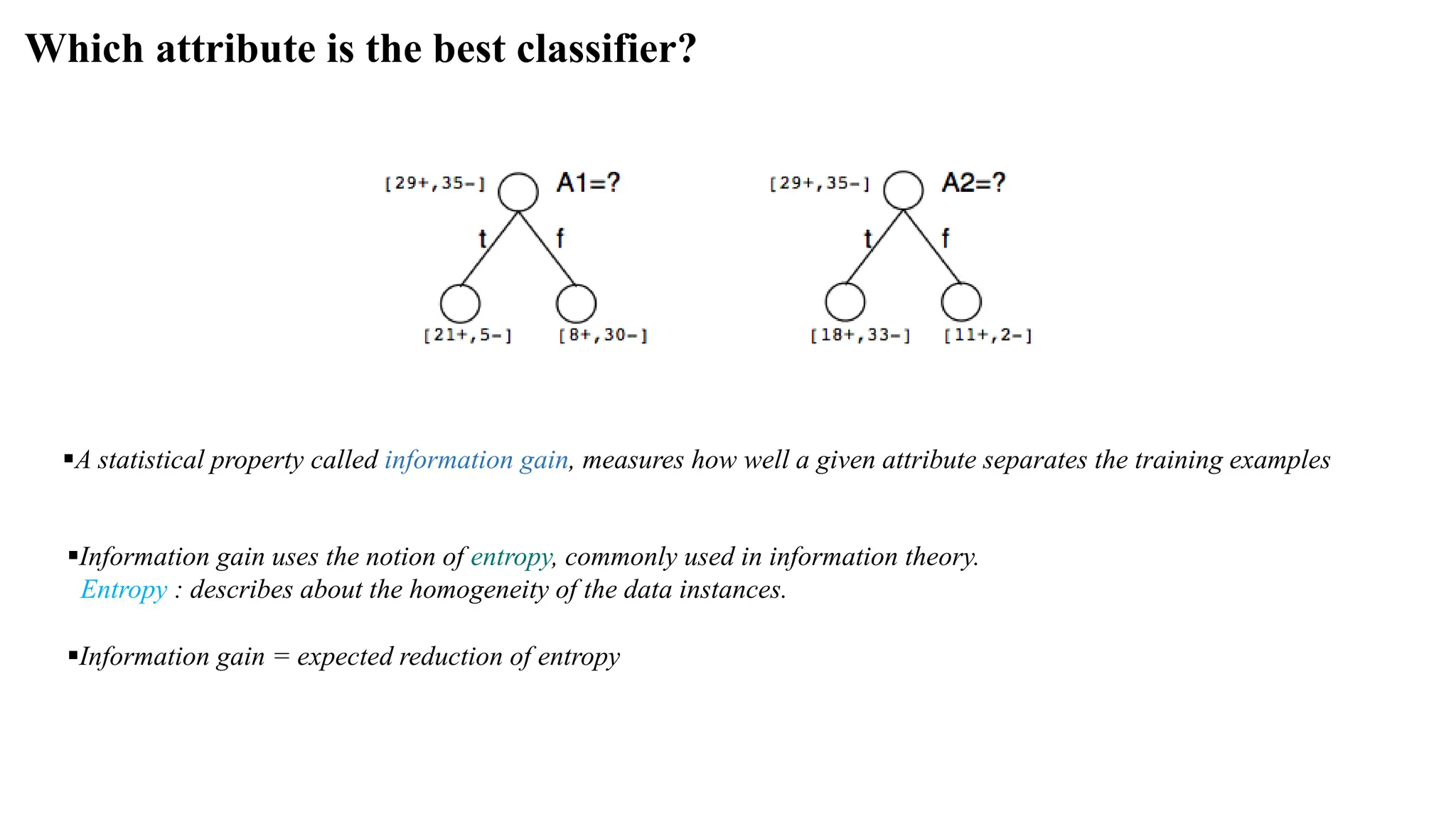
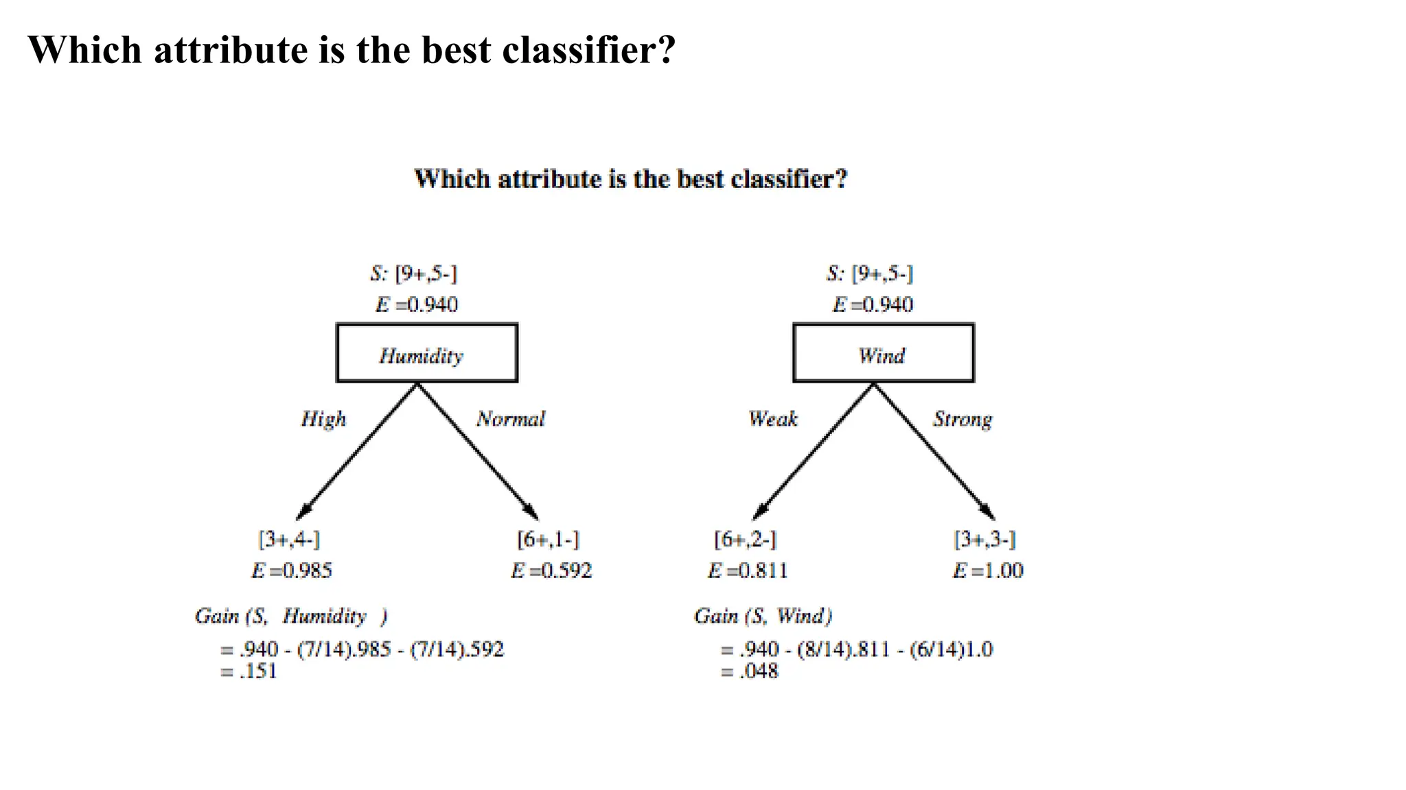
Which attribute isthe best classifier?
A statistical property called information gain, measures how well a given attribute separates the training examples
Information gain uses the notion of entropy, commonly used in information theory.
Entropy : describes about the homogeneity of the data instances.
Information gain = expected reduction of entropy
13.
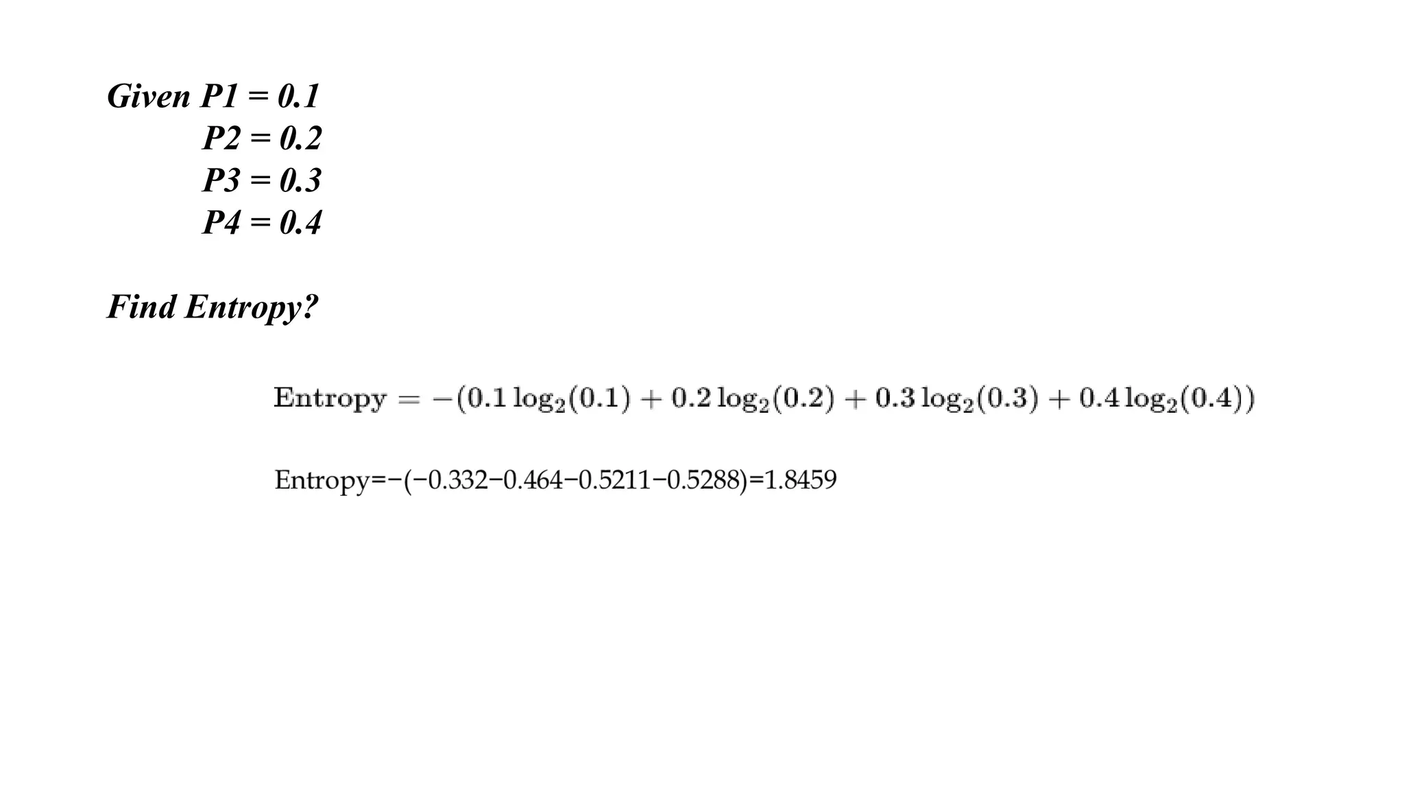
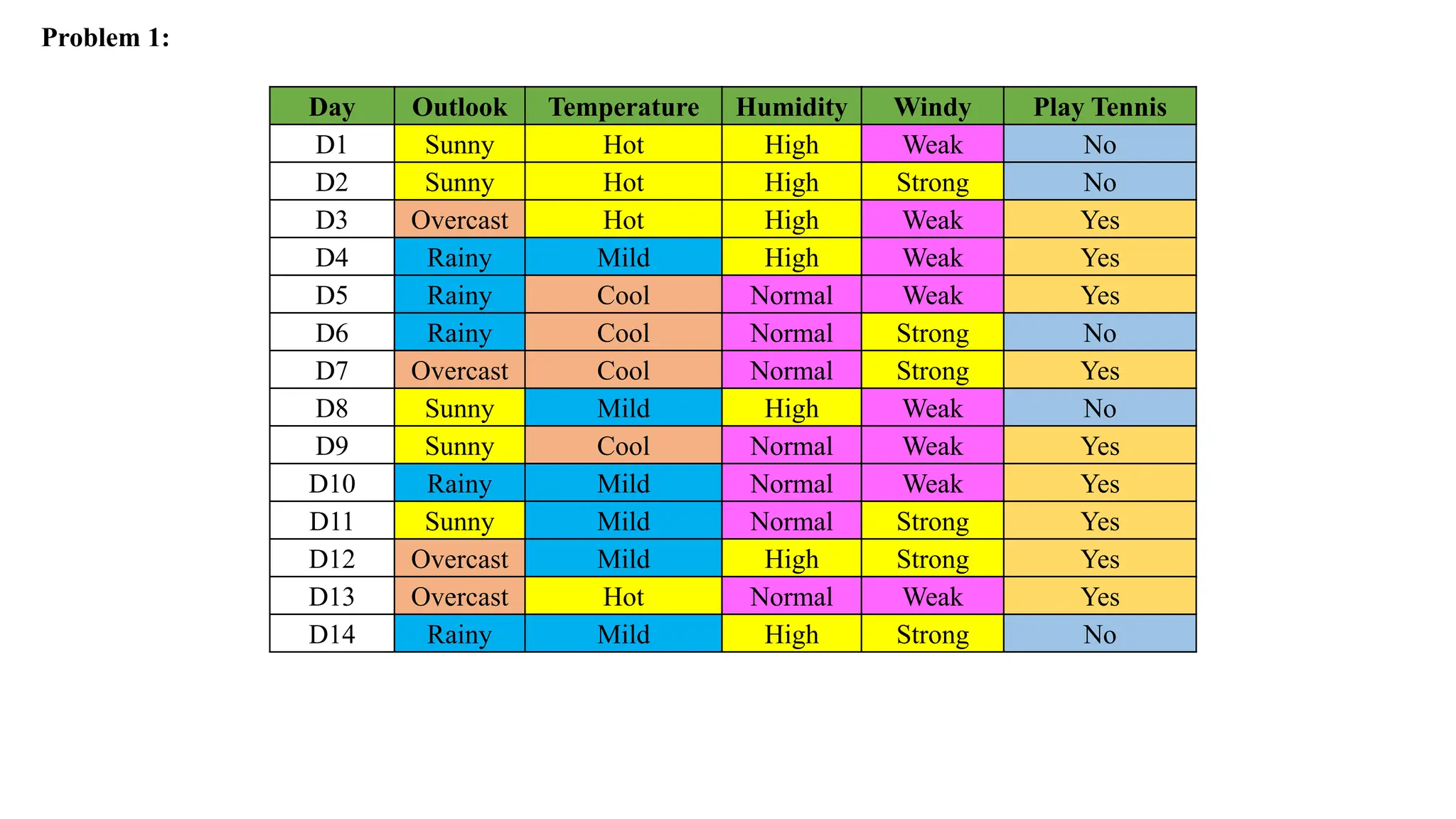
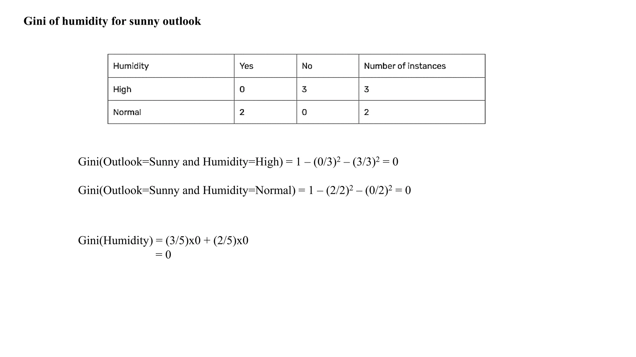
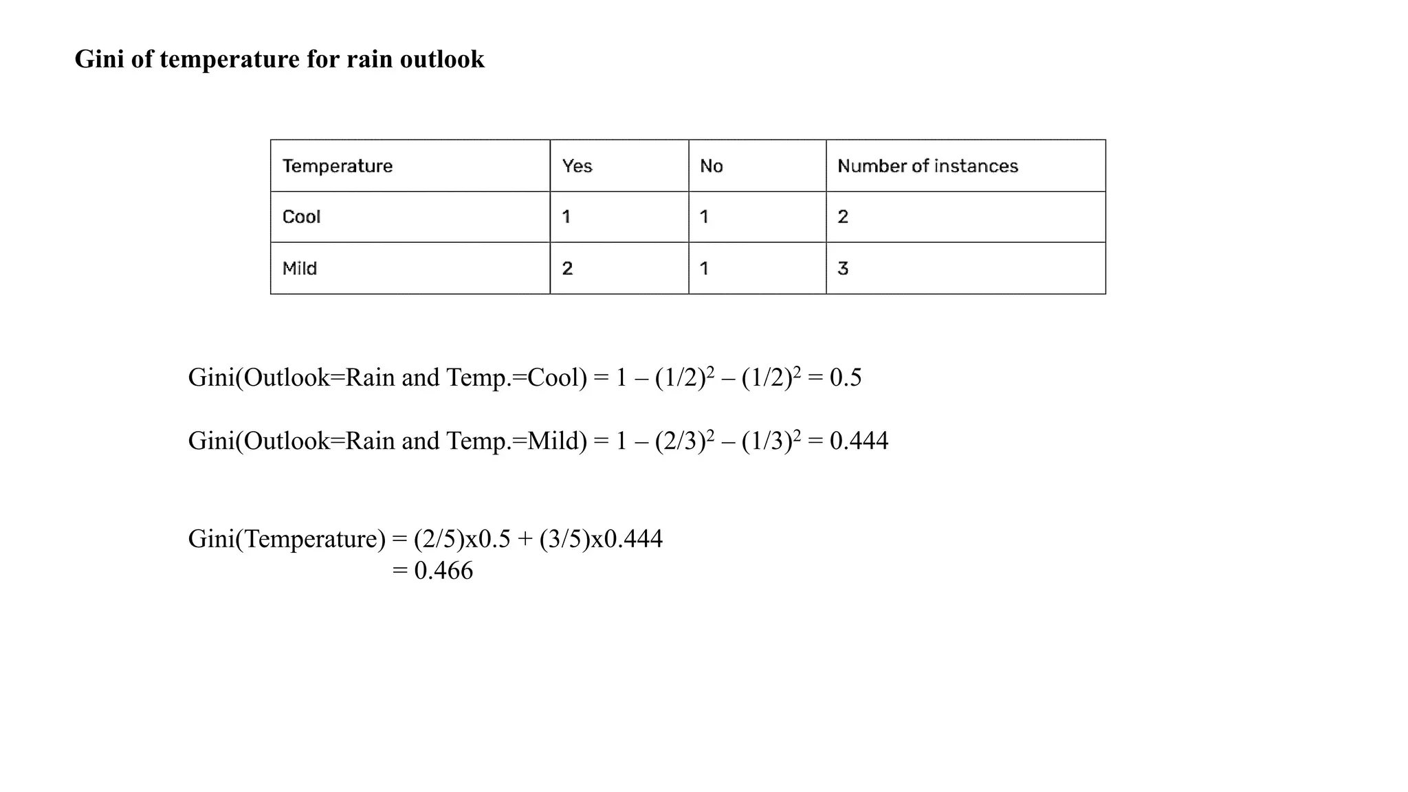
Entropy in binaryclassification
Entropy measures the impurity of a collection of examples.
It depends from the distribution of the random variable p.
S is a collection of training examples
p+ the proportion of positive examples in S
p– the proportion of negative examples in S
Entropy (S) – p+ log2 p+ – p– log2 p– [0 log20 = 0]
Entropy ([14+, 0–]) = – 14/14 log2 (14/14) – 0 log2 (0) = 0
Entropy ([9+, 5–]) = – 9/14 log2 (9/14) – 5/14 log2 (5/14) = 0.94
Entropy ([7+, 7– ]) = – 7/14 log2 (7/14) – 7/14 log2 (7/14) = 1/2 + 1/2 = 1
Note: the log of a number < 1 is negative, 0 p 1, 0 entropy 1
14.
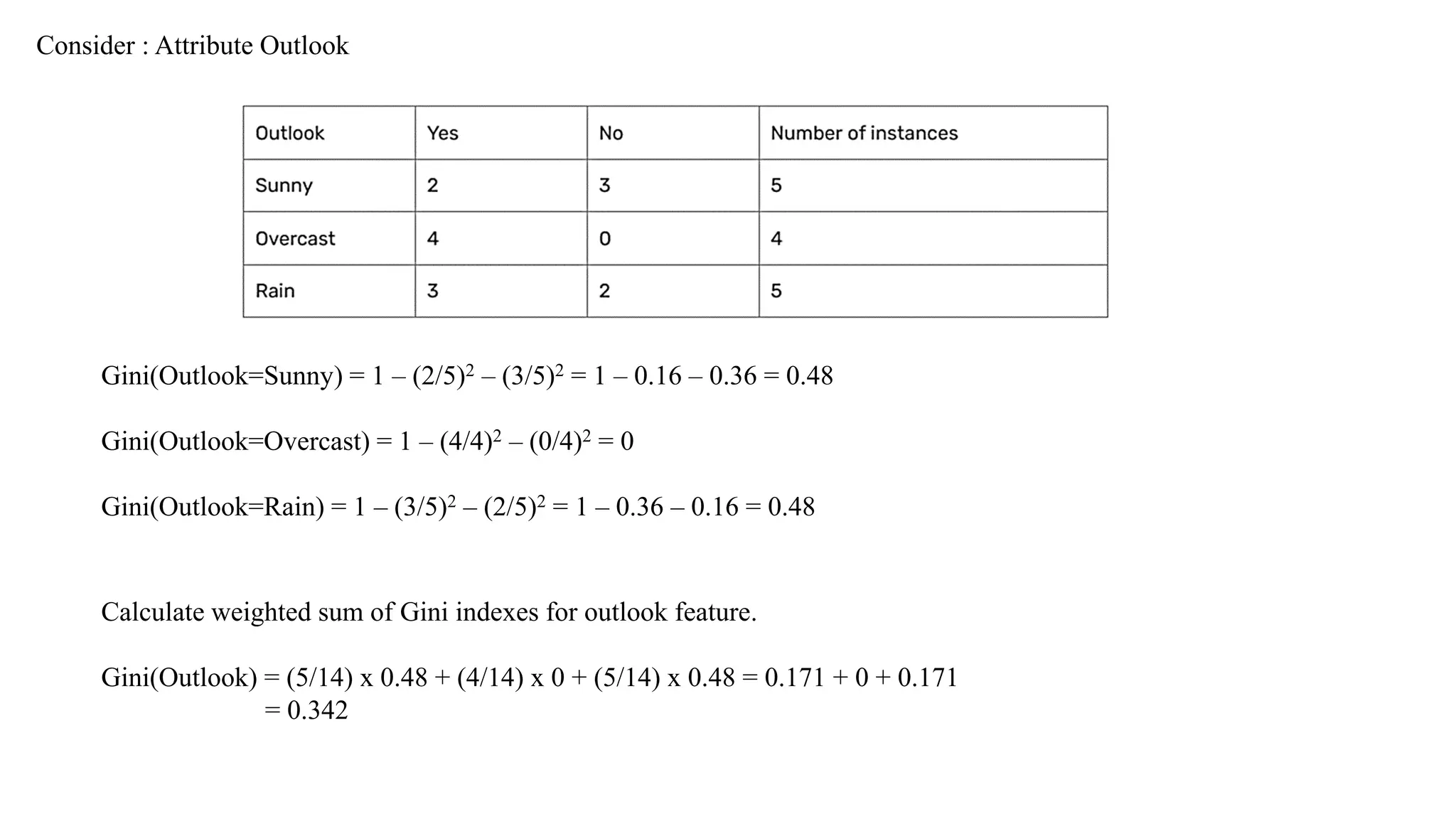
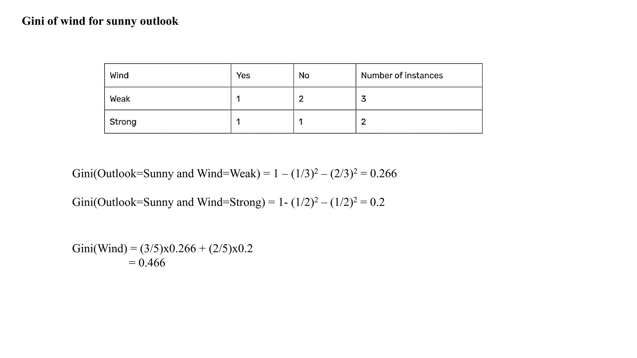
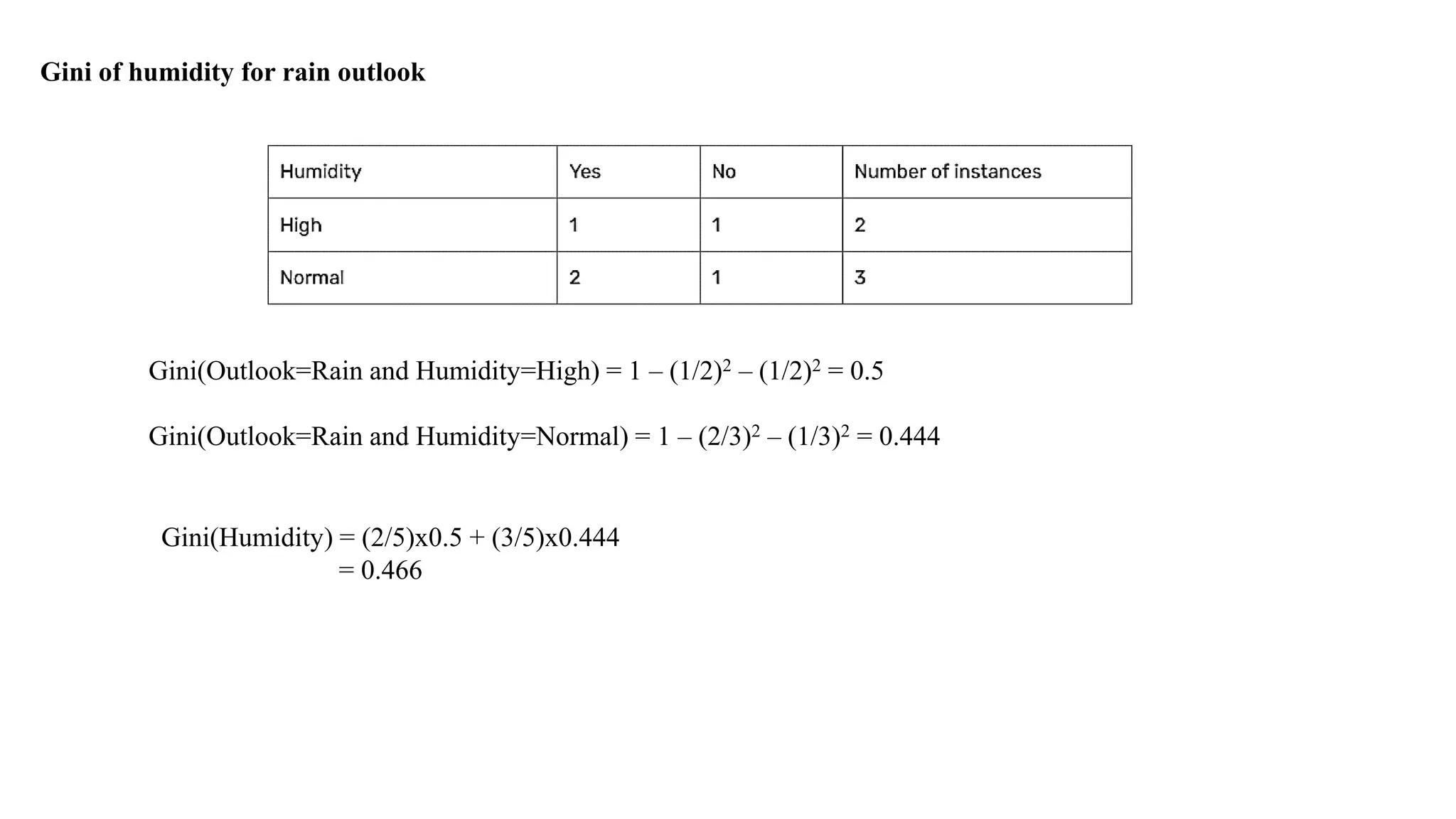
Entropy in general
•Entropy measures the amount of information in a random variable
H(X) = – p+ log2 p+ – p– log2 p– X = {+, –}
for binary classification [two-valued random variable]
c c
H(X) = – pi log2 pi = pi log2 1/ pi X = {i, …, c}
i=1 i=1
for classification in c classes
Example: rolling a die with 8, equally probable, sides
8
H(X) = – 1/8 log2 1/8 = – log2 1/8 = log2 8 = 3
i=1
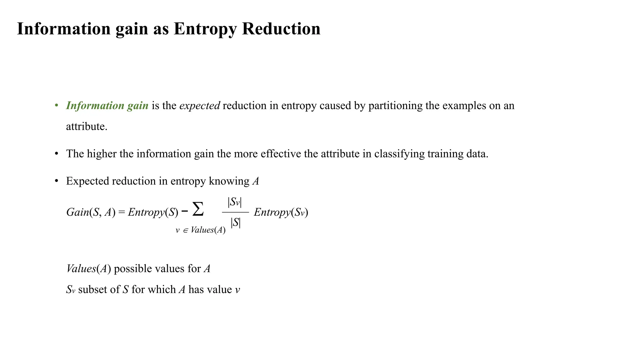
Information gain asEntropy Reduction
• Information gain is the expected reduction in entropy caused by partitioning the examples on an
attribute.
• The higher the information gain the more effective the attribute in classifying training data.
• Expected reduction in entropy knowing A
Gain(S, A) = Entropy(S) − Entropy(Sv)
v Values(A)
Values(A) possible values for A
Sv subset of S for which A has value v
|Sv|
|S|
18.
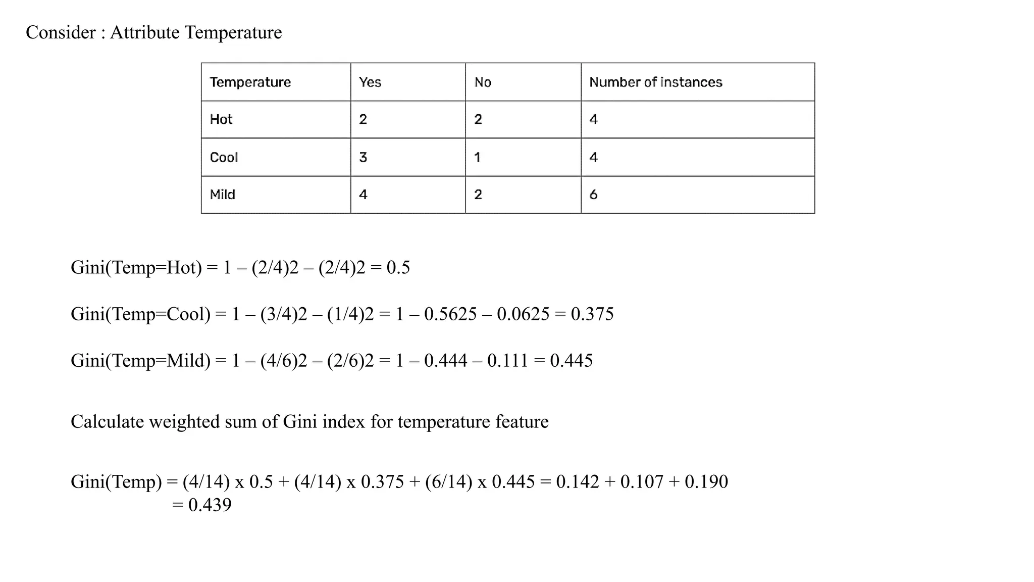
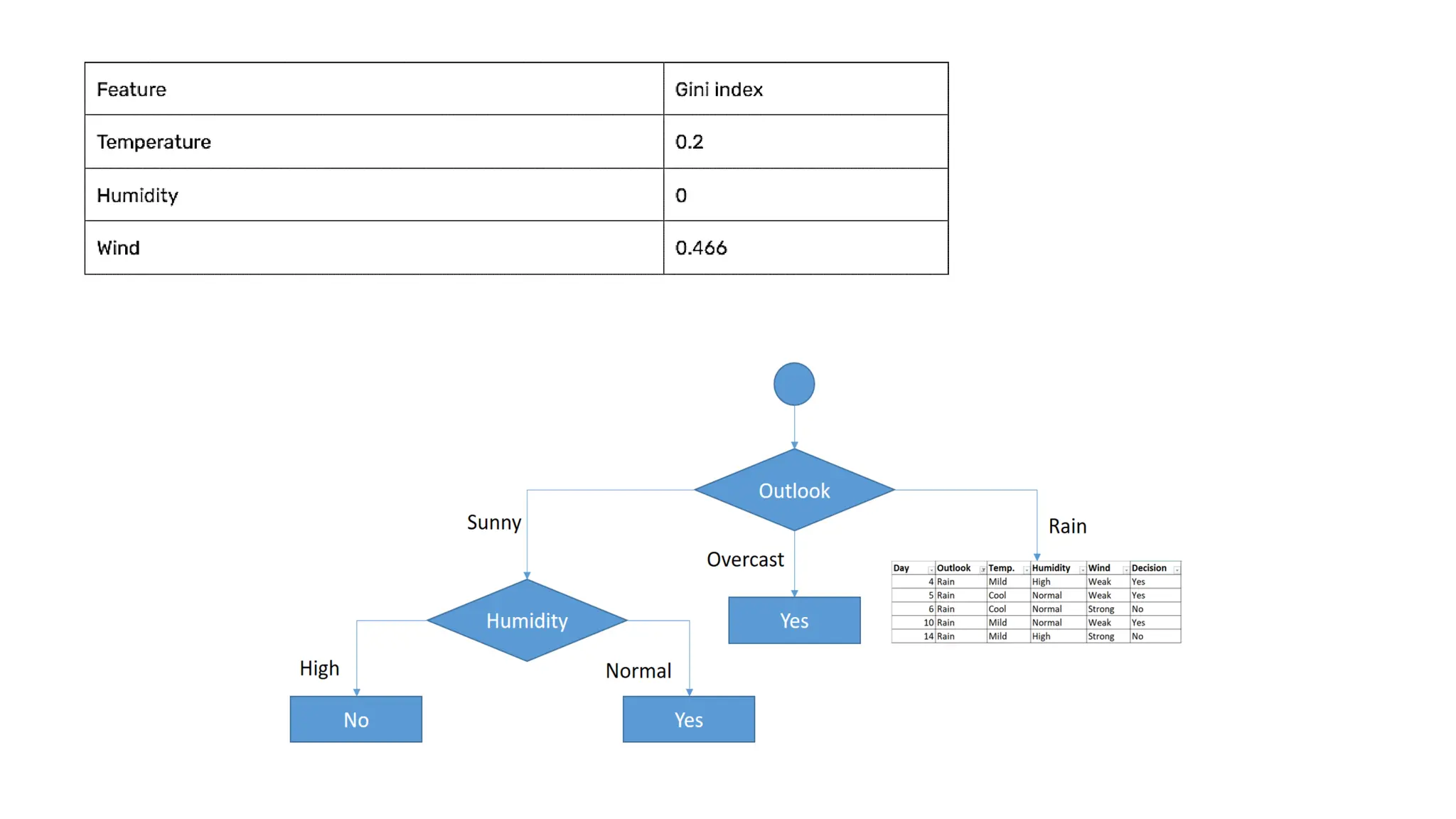
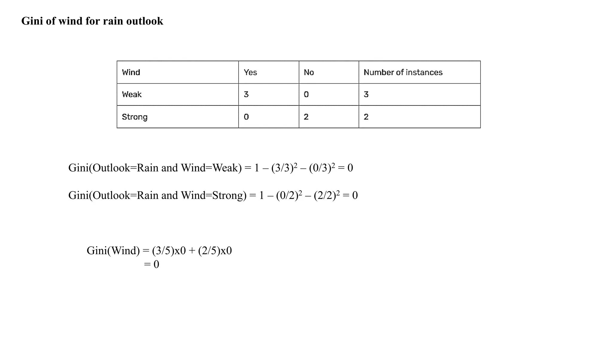
Example: Expected InformationGain
Let
Values(Wind) = {Weak, Strong}
S = [9+, 5−]
SWeak = [6+, 2−]
SStrong = [3+, 3−]
Information gain due to knowing Wind:
Gain(S, Wind) = Entropy(S) − 8/14 Entropy(SWeak) − 6/14 Entropy(SStrong)
= 0.94 − 8/14 0.811 − 6/14 1.00
= 0.048
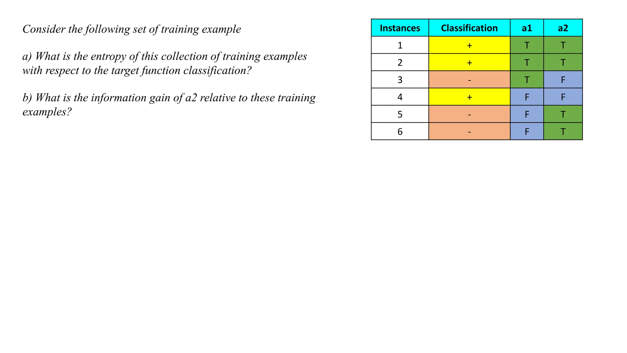
Consider the followingset of training example Instances Classification a1 a2
1 + T T
2 + T T
3 - T F
4 + F F
5 - F T
6 - F T
a) What is the entropy of this collection of training examples
with respect to the target function classification?
b) What is the information gain of a2 relative to these training
examples?
21.
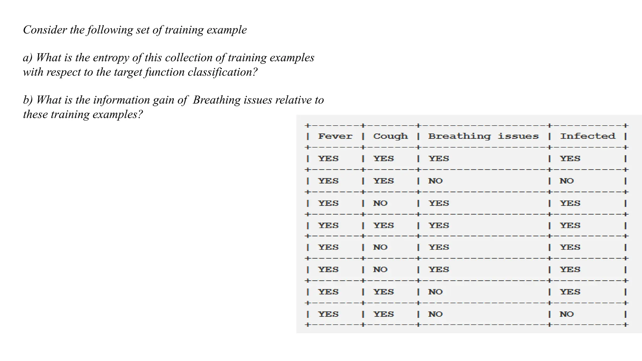
Consider the followingset of training example
a) What is the entropy of this collection of training examples
with respect to the target function classification?
b) What is the information gain of Breathing issues relative to
these training examples?
22.
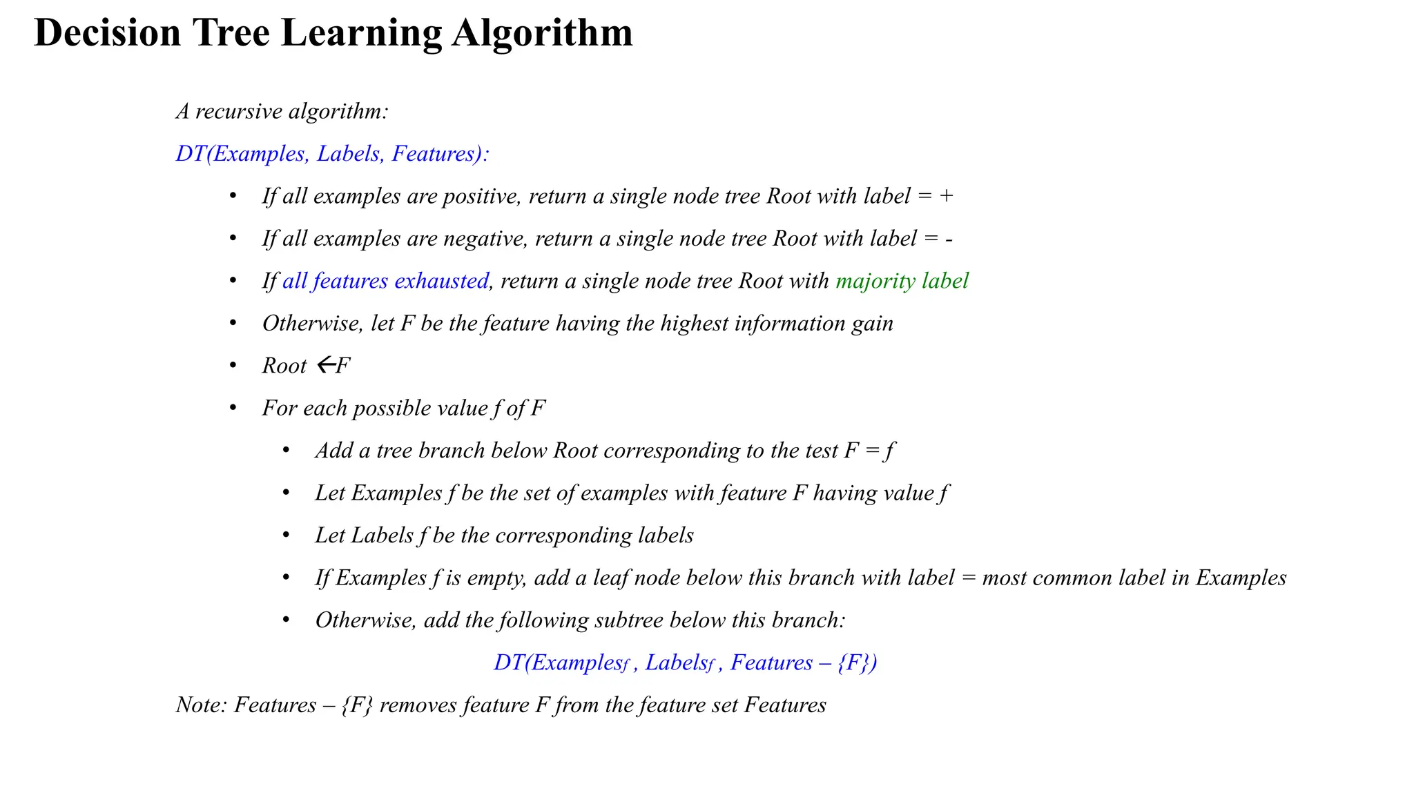
Decision Tree LearningAlgorithm
A recursive algorithm:
DT(Examples, Labels, Features):
• If all examples are positive, return a single node tree Root with label = +
• If all examples are negative, return a single node tree Root with label = -
• If all features exhausted, return a single node tree Root with majority label
• Otherwise, let F be the feature having the highest information gain
• Root F
• For each possible value f of F
• Add a tree branch below Root corresponding to the test F = f
• Let Examples f be the set of examples with feature F having value f
• Let Labels f be the corresponding labels
• If Examples f is empty, add a leaf node below this branch with label = most common label in Examples
• Otherwise, add the following subtree below this branch:
DT(Examplesf , Labelsf , Features – {F})
Note: Features – {F} removes feature F from the feature set Features
23.
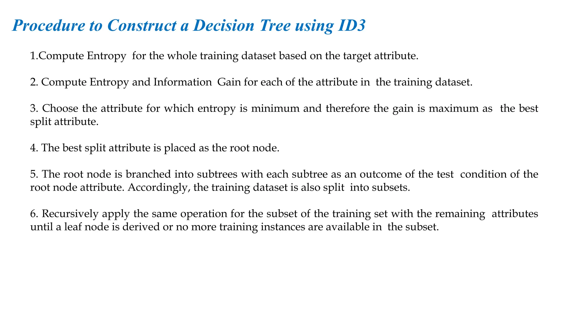
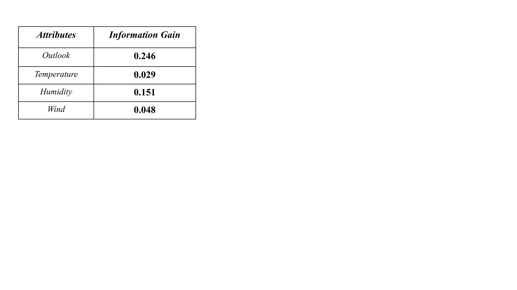
1.Compute Entropy forthe whole training dataset based on the target attribute.
2. Compute Entropy and Information Gain for each of the attribute in the training dataset.
3. Choose the attribute for which entropy is minimum and therefore the gain is maximum as the best
split attribute.
4. The best split attribute is placed as the root node.
5. The root node is branched into subtrees with each subtree as an outcome of the test condition of the
root node attribute. Accordingly, the training dataset is also split into subsets.
6. Recursively apply the same operation for the subset of the training set with the remaining attributes
until a leaf node is derived or no more training instances are available in the subset.
Procedure to Construct a Decision Tree using ID3
24.
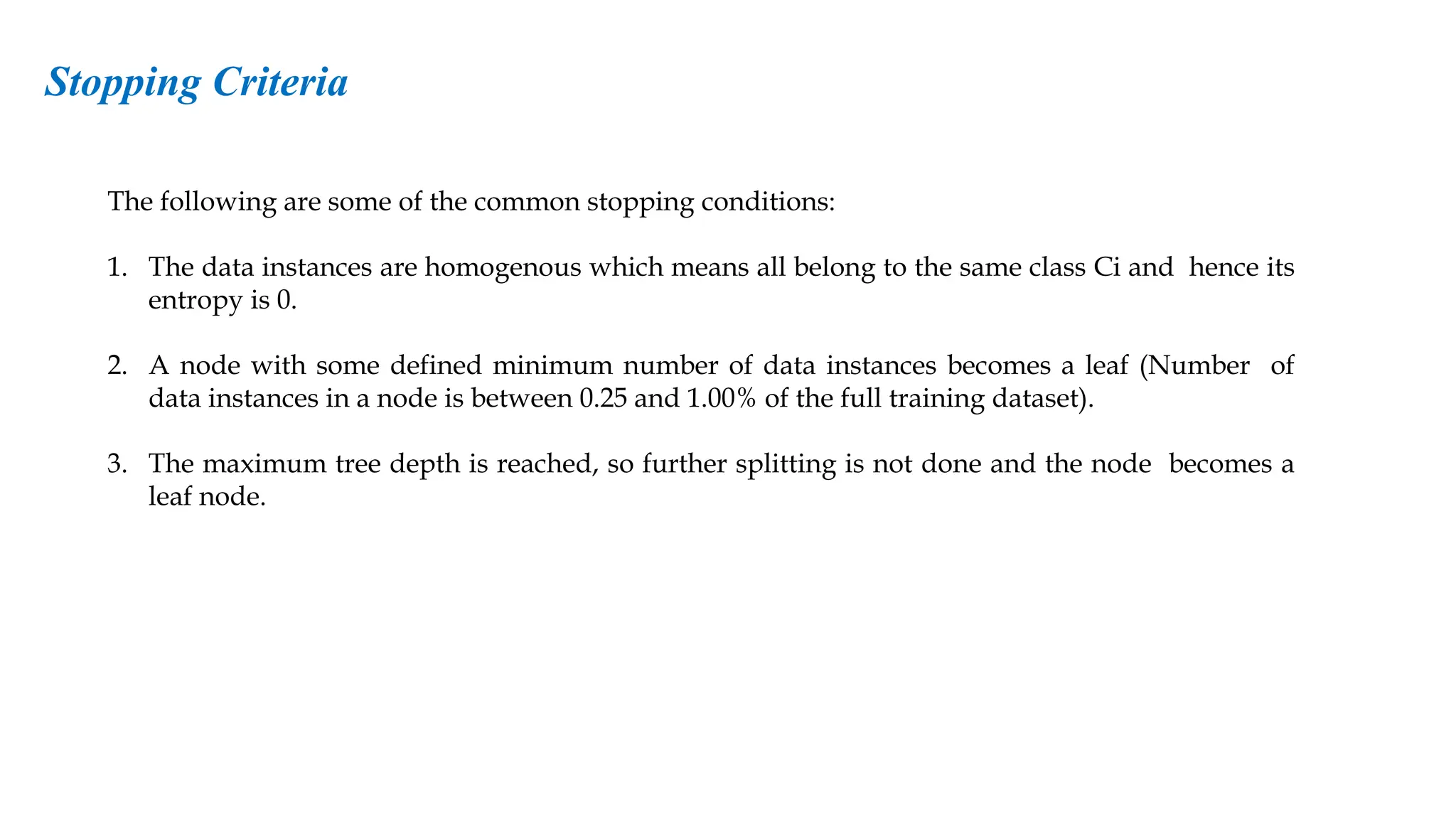
The following aresome of the common stopping conditions:
1. The data instances are homogenous which means all belong to the same class Ci and hence its
entropy is 0.
2. A node with some defined minimum number of data instances becomes a leaf (Number of
data instances in a node is between 0.25 and 1.00% of the full training dataset).
3. The maximum tree depth is reached, so further splitting is not done and the node becomes a
leaf node.
Stopping Criteria
25.
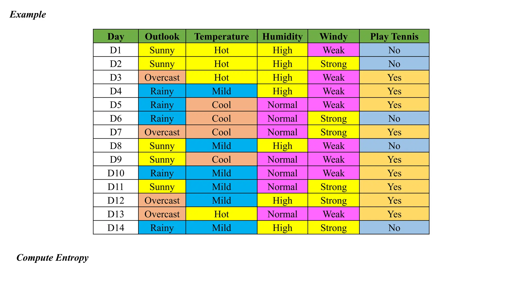
Day Outlook TemperatureHumidity Windy Play Tennis
D1 Sunny Hot High Weak No
D2 Sunny Hot High Strong No
D3 Overcast Hot High Weak Yes
D4 Rainy Mild High Weak Yes
D5 Rainy Cool Normal Weak Yes
D6 Rainy Cool Normal Strong No
D7 Overcast Cool Normal Strong Yes
D8 Sunny Mild High Weak No
D9 Sunny Cool Normal Weak Yes
D10 Rainy Mild Normal Weak Yes
D11 Sunny Mild Normal Strong Yes
D12 Overcast Mild High Strong Yes
D13 Overcast Hot Normal Weak Yes
D14 Rainy Mild High Strong No
Compute Entropy
Example
26.
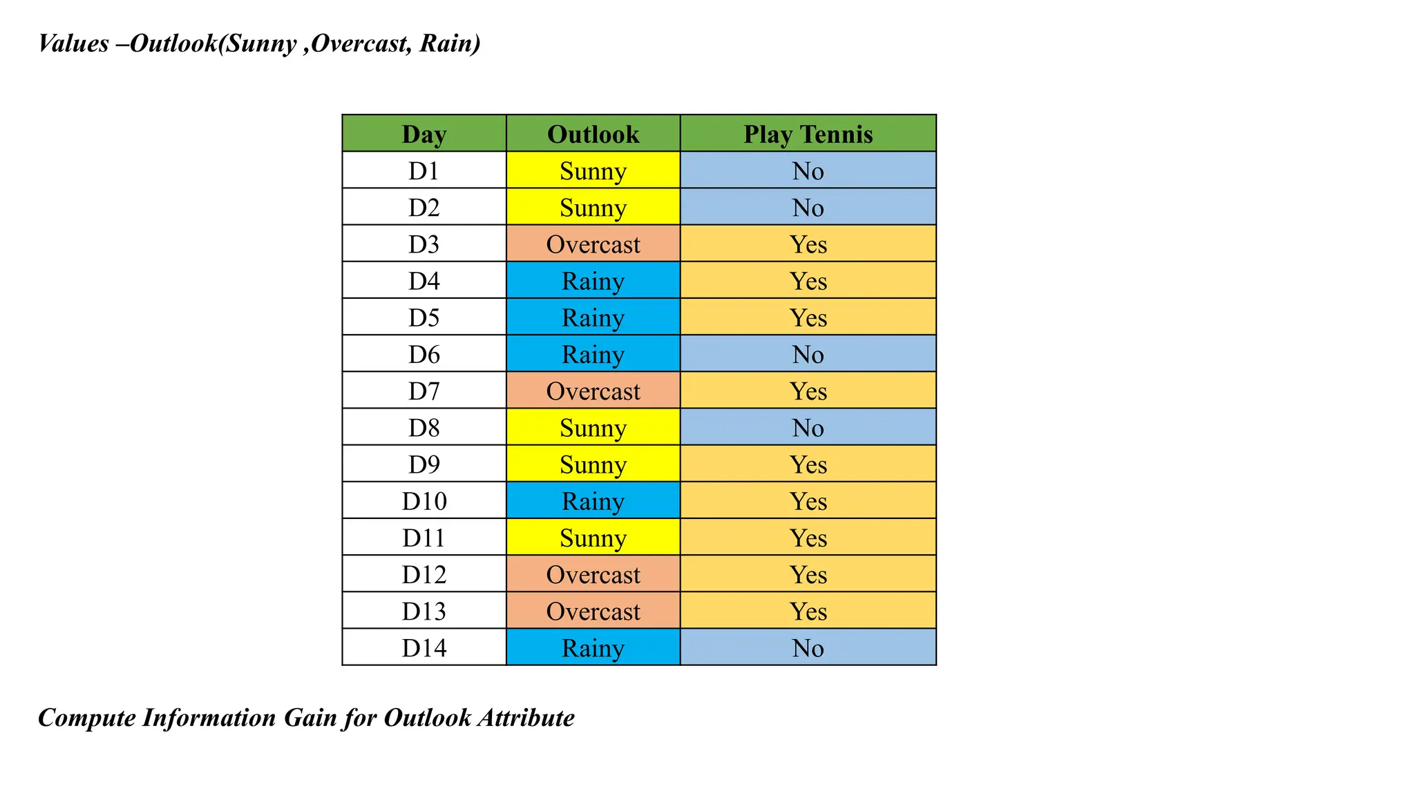
Day Outlook PlayTennis
D1 Sunny No
D2 Sunny No
D3 Overcast Yes
D4 Rainy Yes
D5 Rainy Yes
D6 Rainy No
D7 Overcast Yes
D8 Sunny No
D9 Sunny Yes
D10 Rainy Yes
D11 Sunny Yes
D12 Overcast Yes
D13 Overcast Yes
D14 Rainy No
Values –Outlook(Sunny ,Overcast, Rain)
Compute Information Gain for Outlook Attribute
27.
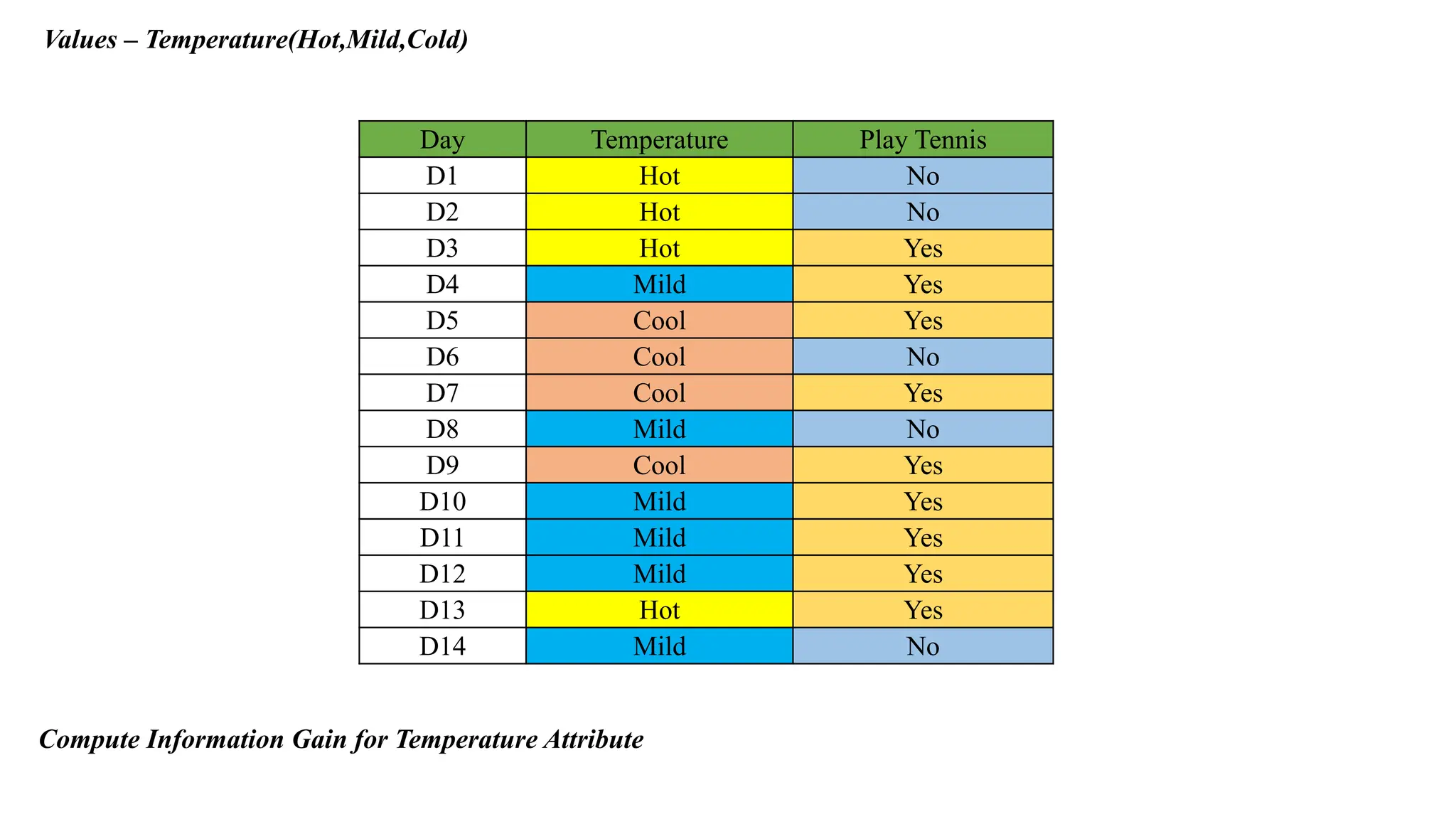
Values – Temperature(Hot,Mild,Cold)
DayTemperature Play Tennis
D1 Hot No
D2 Hot No
D3 Hot Yes
D4 Mild Yes
D5 Cool Yes
D6 Cool No
D7 Cool Yes
D8 Mild No
D9 Cool Yes
D10 Mild Yes
D11 Mild Yes
D12 Mild Yes
D13 Hot Yes
D14 Mild No
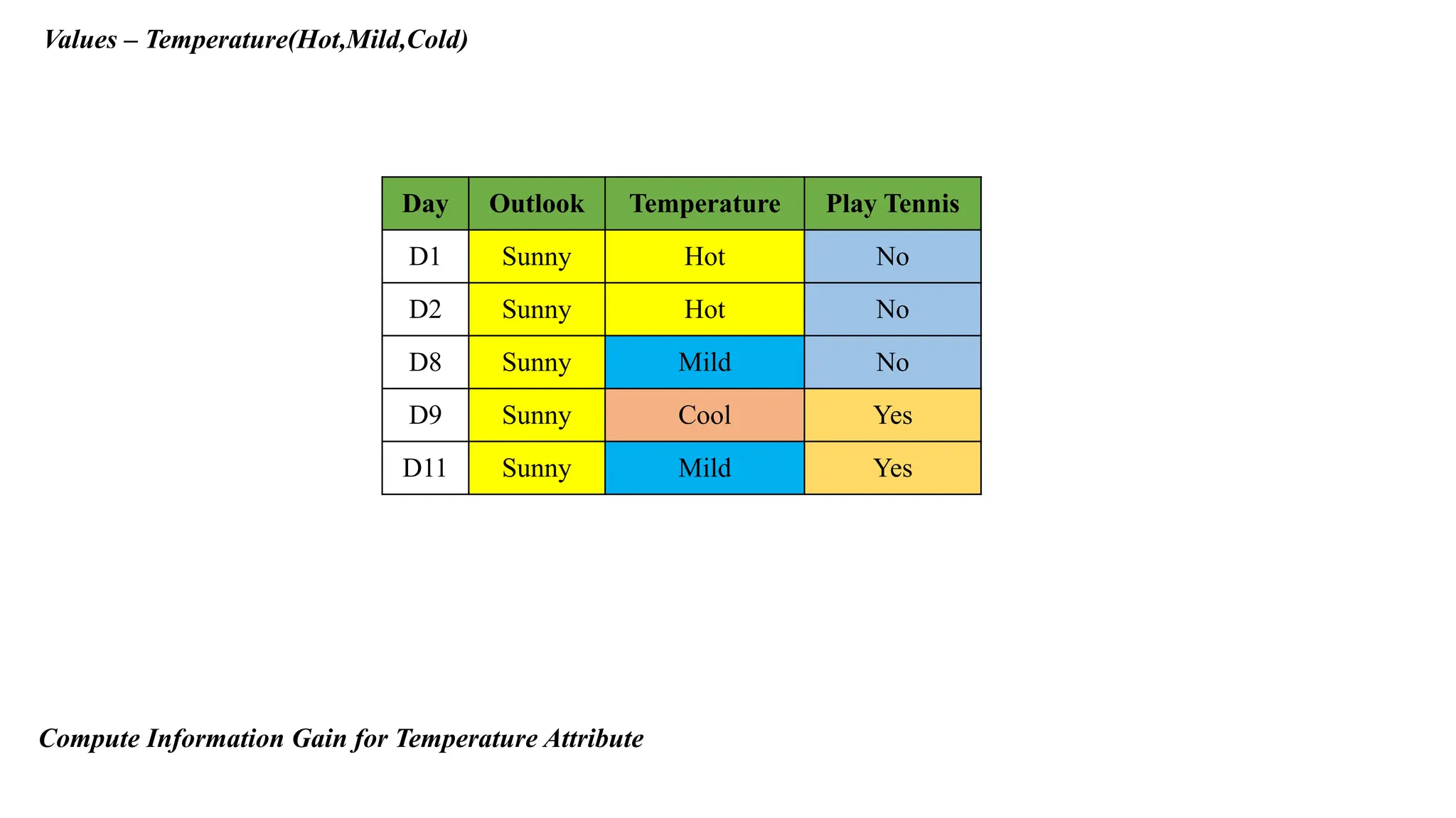
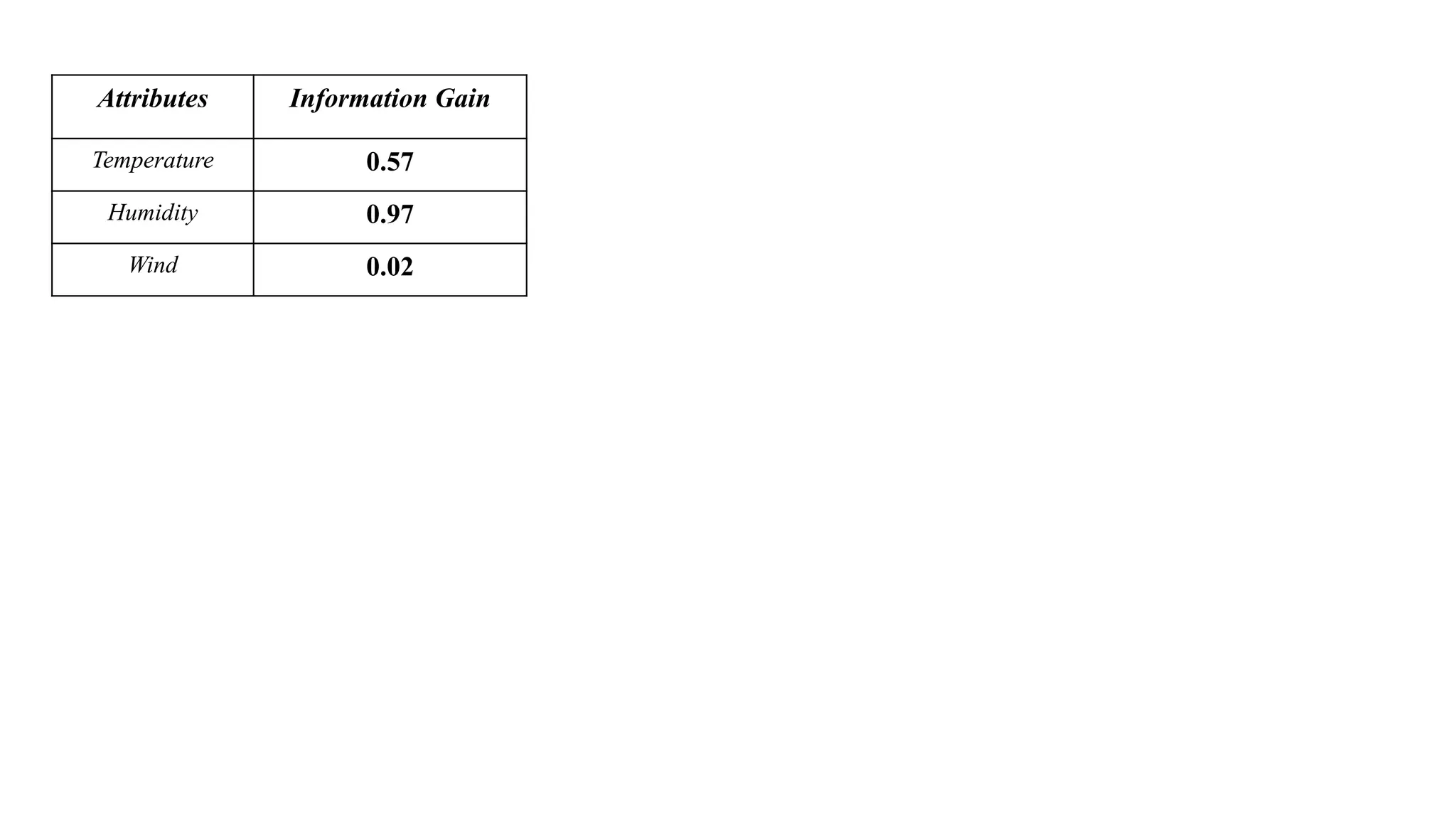
Compute Information Gain for Temperature Attribute
28.
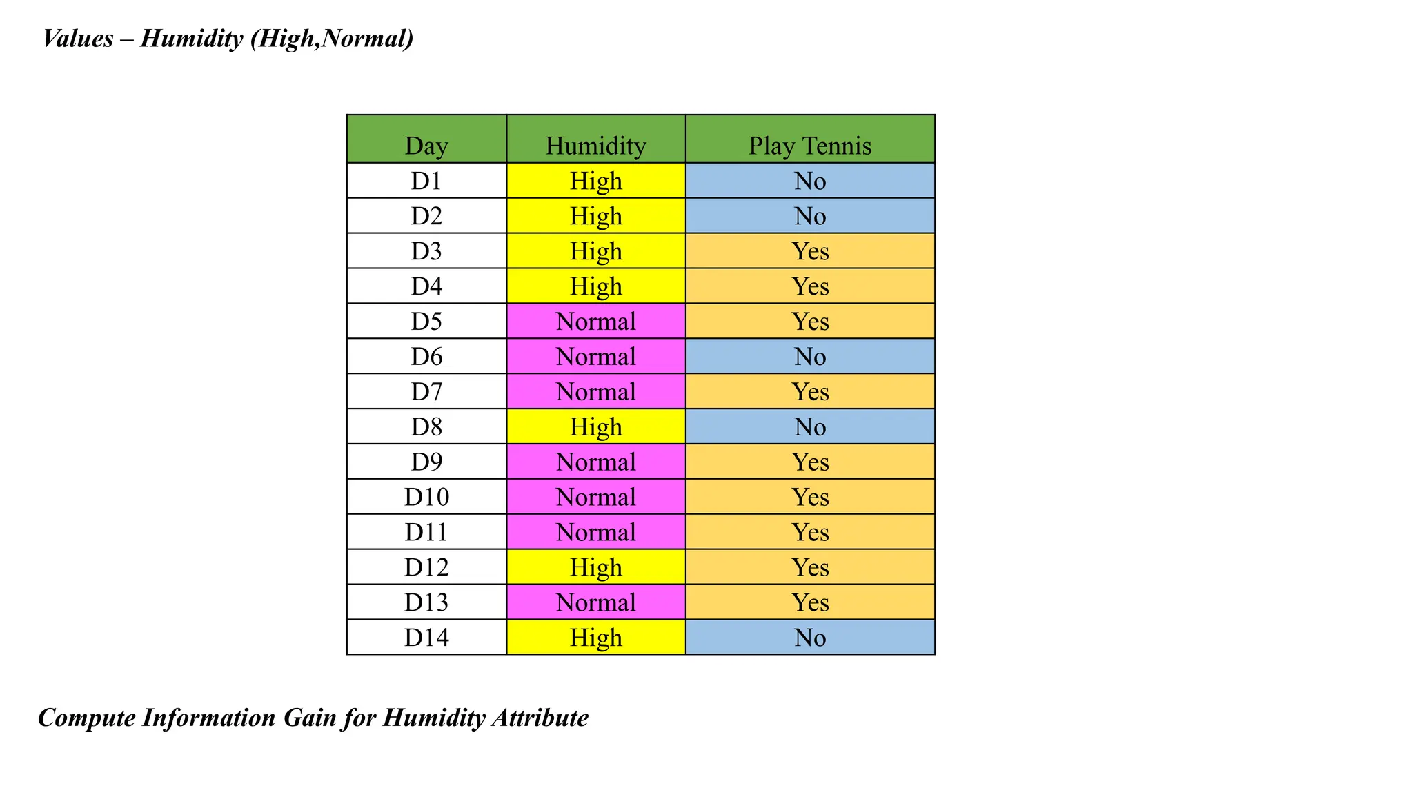
Values – Humidity(High,Normal)
Day Humidity Play Tennis
D1 High No
D2 High No
D3 High Yes
D4 High Yes
D5 Normal Yes
D6 Normal No
D7 Normal Yes
D8 High No
D9 Normal Yes
D10 Normal Yes
D11 Normal Yes
D12 High Yes
D13 Normal Yes
D14 High No
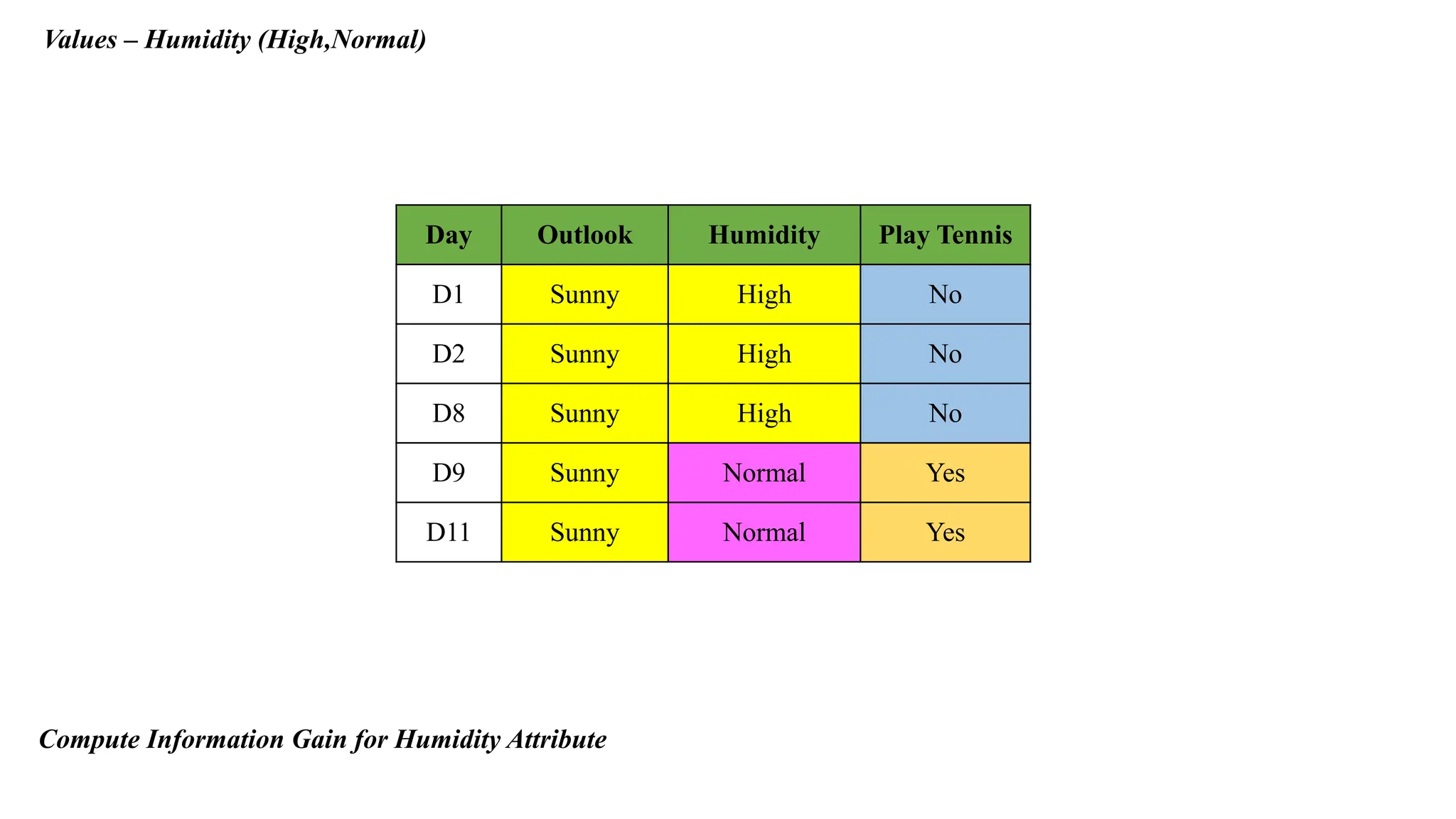
Compute Information Gain for Humidity Attribute
29.
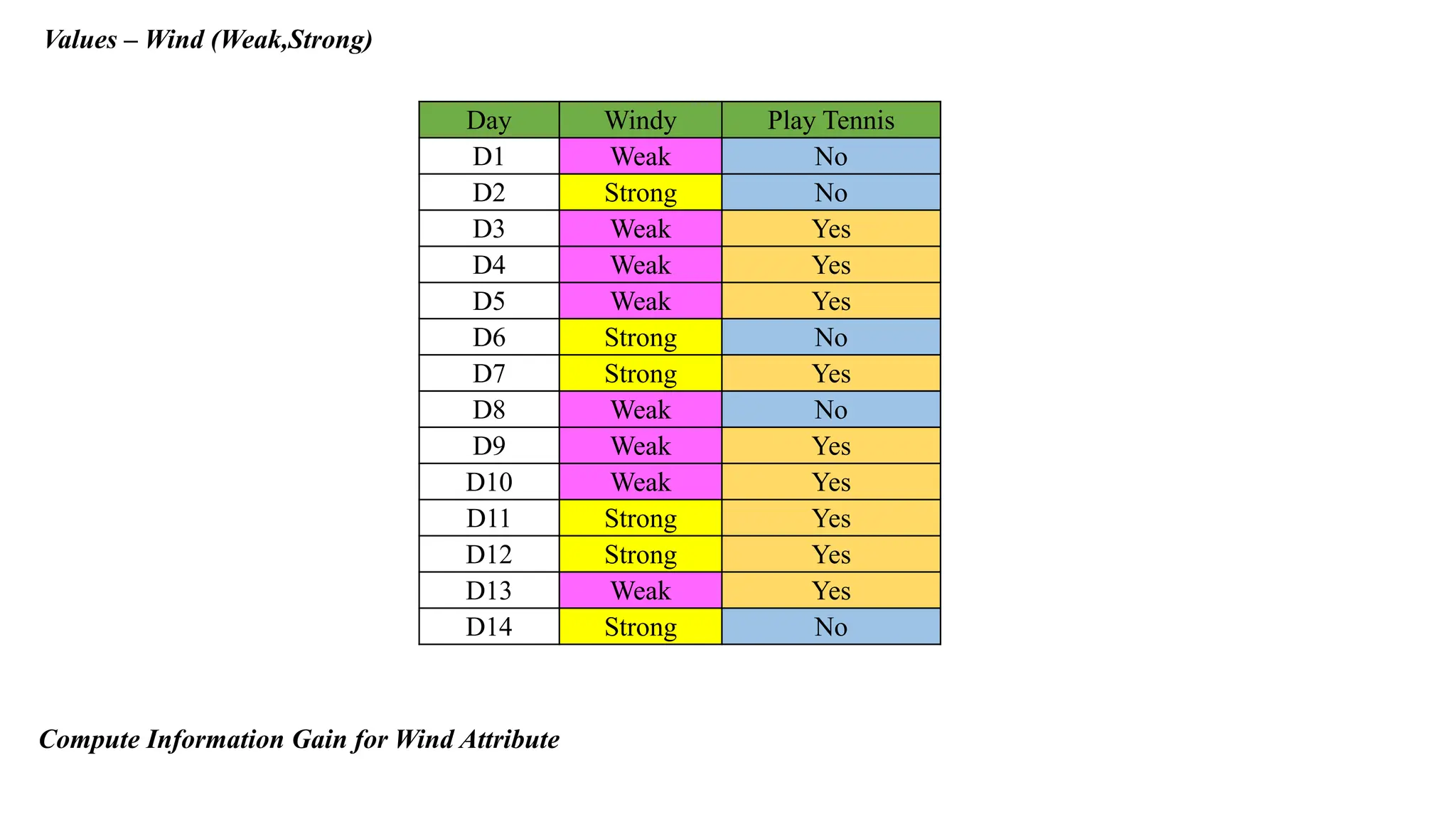
Values – Wind(Weak,Strong)
Day Windy Play Tennis
D1 Weak No
D2 Strong No
D3 Weak Yes
D4 Weak Yes
D5 Weak Yes
D6 Strong No
D7 Strong Yes
D8 Weak No
D9 Weak Yes
D10 Weak Yes
D11 Strong Yes
D12 Strong Yes
D13 Weak Yes
D14 Strong No
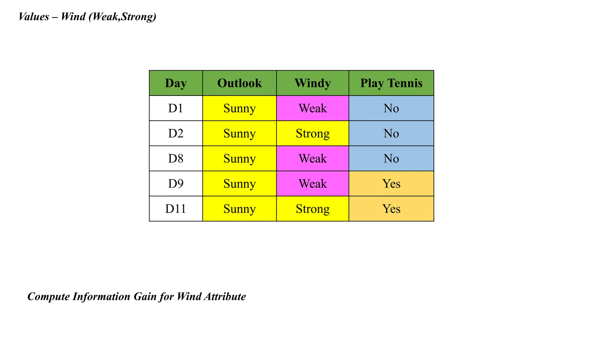
Compute Information Gain for Wind Attribute
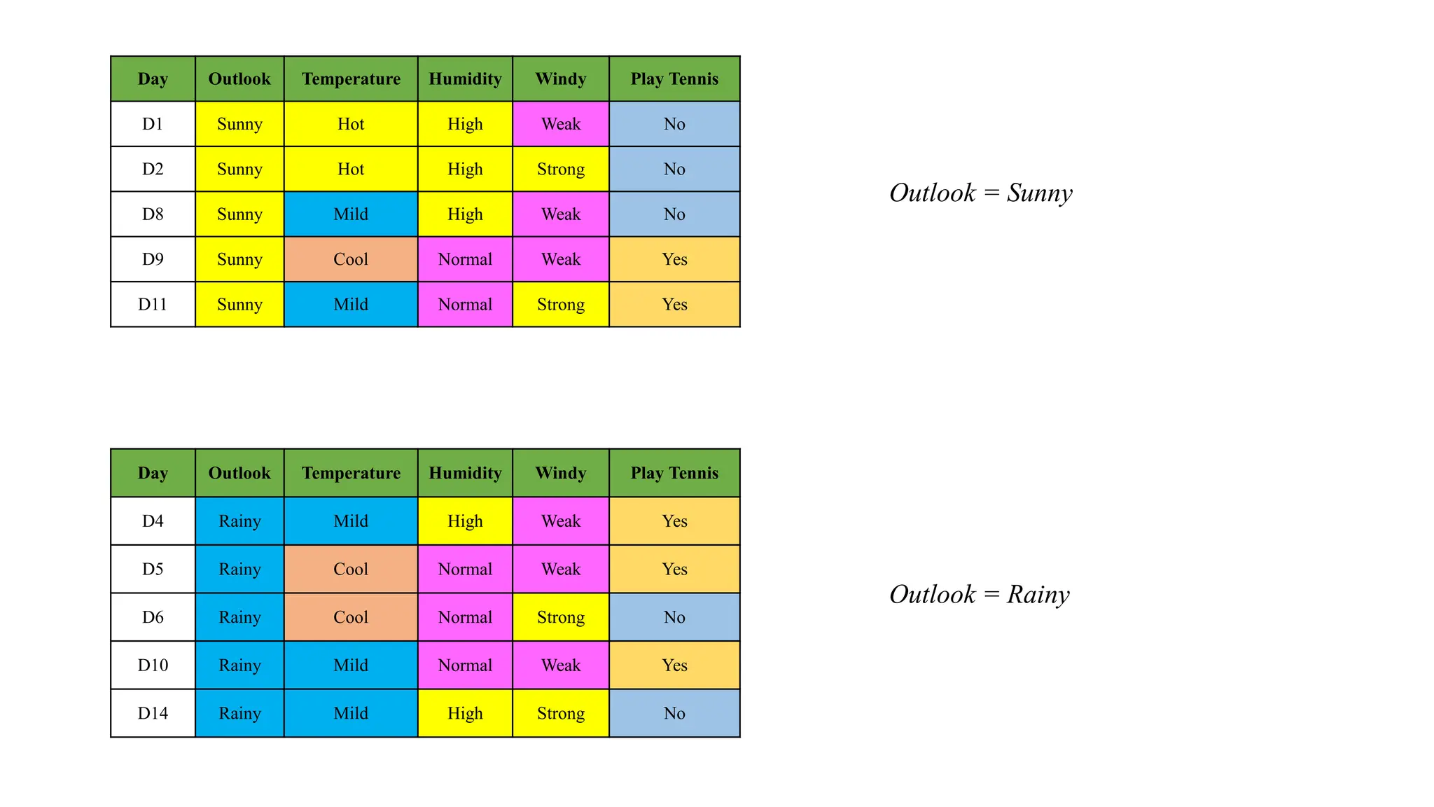
Day Outlook TemperatureHumidity Windy Play Tennis
D1 Sunny Hot High Weak No
D2 Sunny Hot High Strong No
D8 Sunny Mild High Weak No
D9 Sunny Cool Normal Weak Yes
D11 Sunny Mild Normal Strong Yes
Outlook = Sunny
Day Outlook Temperature Humidity Windy Play Tennis
D4 Rainy Mild High Weak Yes
D5 Rainy Cool Normal Weak Yes
D6 Rainy Cool Normal Strong No
D10 Rainy Mild Normal Weak Yes
D14 Rainy Mild High Strong No
Outlook = Rainy
32.
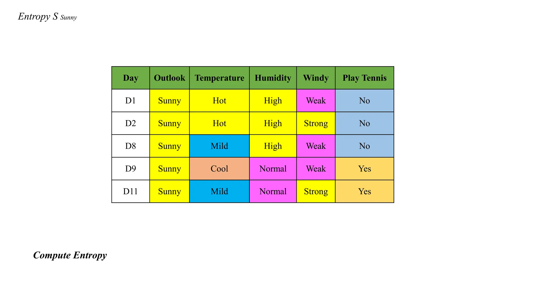
Entropy S Sunny
DayOutlook Temperature Humidity Windy Play Tennis
D1 Sunny Hot High Weak No
D2 Sunny Hot High Strong No
D8 Sunny Mild High Weak No
D9 Sunny Cool Normal Weak Yes
D11 Sunny Mild Normal Strong Yes
Compute Entropy
33.
Values – Temperature(Hot,Mild,Cold)
DayOutlook Temperature Play Tennis
D1 Sunny Hot No
D2 Sunny Hot No
D8 Sunny Mild No
D9 Sunny Cool Yes
D11 Sunny Mild Yes
Compute Information Gain for Temperature Attribute
34.
Values – Humidity(High,Normal)
Day Outlook Humidity Play Tennis
D1 Sunny High No
D2 Sunny High No
D8 Sunny High No
D9 Sunny Normal Yes
D11 Sunny Normal Yes
Compute Information Gain for Humidity Attribute
35.
Values – Wind(Weak,Strong)
Day Outlook Windy Play Tennis
D1 Sunny Weak No
D2 Sunny Strong No
D8 Sunny Weak No
D9 Sunny Weak Yes
D11 Sunny Strong Yes
Compute Information Gain for Wind Attribute
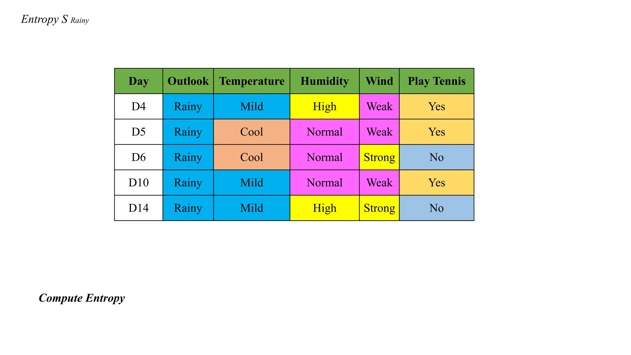
Entropy S Rainy
DayOutlook Temperature Humidity Wind Play Tennis
D4 Rainy Mild High Weak Yes
D5 Rainy Cool Normal Weak Yes
D6 Rainy Cool Normal Strong No
D10 Rainy Mild Normal Weak Yes
D14 Rainy Mild High Strong No
Compute Entropy
38.
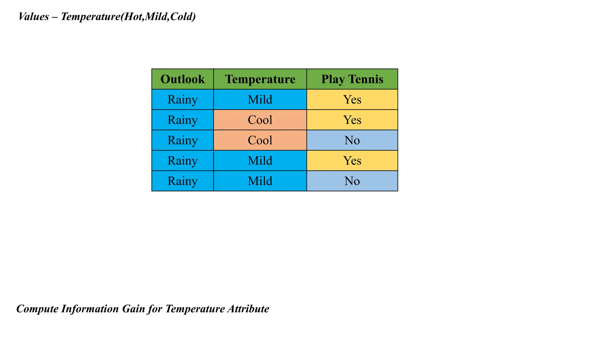
Values – Temperature(Hot,Mild,Cold)
OutlookTemperature Play Tennis
Rainy Mild Yes
Rainy Cool Yes
Rainy Cool No
Rainy Mild Yes
Rainy Mild No
Compute Information Gain for Temperature Attribute
39.
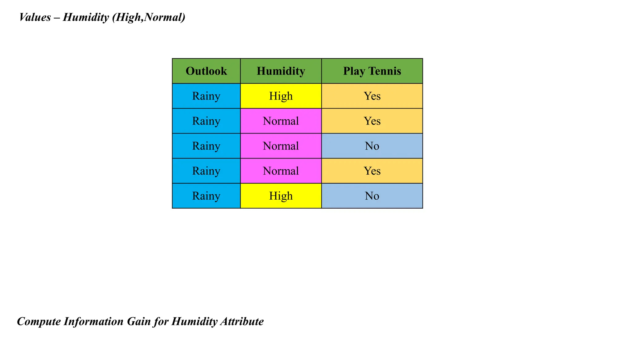
Values – Humidity(High,Normal)
Outlook Humidity Play Tennis
Rainy High Yes
Rainy Normal Yes
Rainy Normal No
Rainy Normal Yes
Rainy High No
Compute Information Gain for Humidity Attribute
40.
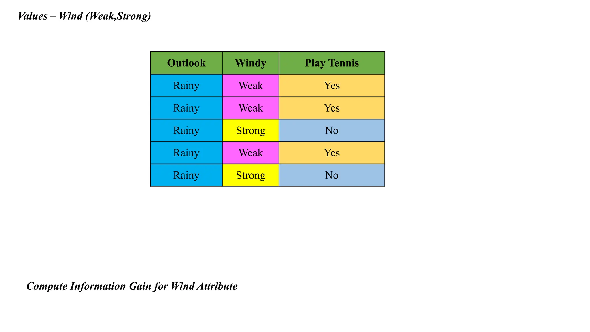
Values – Wind(Weak,Strong)
Outlook Windy Play Tennis
Rainy Weak Yes
Rainy Weak Yes
Rainy Strong No
Rainy Weak Yes
Rainy Strong No
Compute Information Gain for Wind Attribute
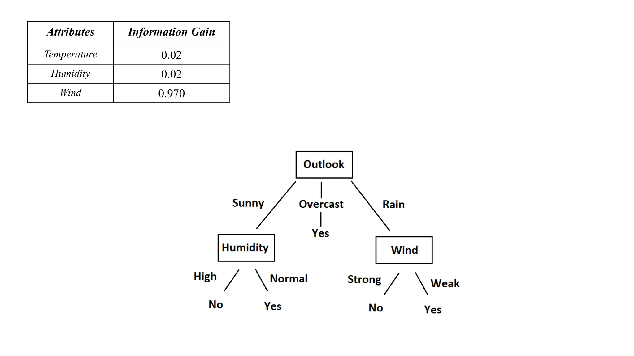
C4.5 is animprovement over ID3.
C4.5 works with continuous and discrete attributes and missing values, and it also supports post-pruning.
C5.0 is the successor of C4.5 and is more efficient and used for building smaller decision trees.
C4.5 works with missing values by marking as ‘?’, but these missing attribute values are not considered in
the calculations.
It uses Gain Ratio as a measure during the construction of decision trees.
To overcome bias issue, C4.5 uses a purity measure Gain ratio to identify the best split attribute.
In C4.5 algorithm, the Information Gain measure used in ID3 algorithm is normalized by computing another
factor called Split_Info.
This normalized information gain of an attribute called as Gain_Ratio is computed by the ratio of the
calculated Split_Info and Information Gain of each attribute.
Then, the attribute with the highest normalized information gain, that is, highest gain ratio is used as the
splitting criteria.
44.
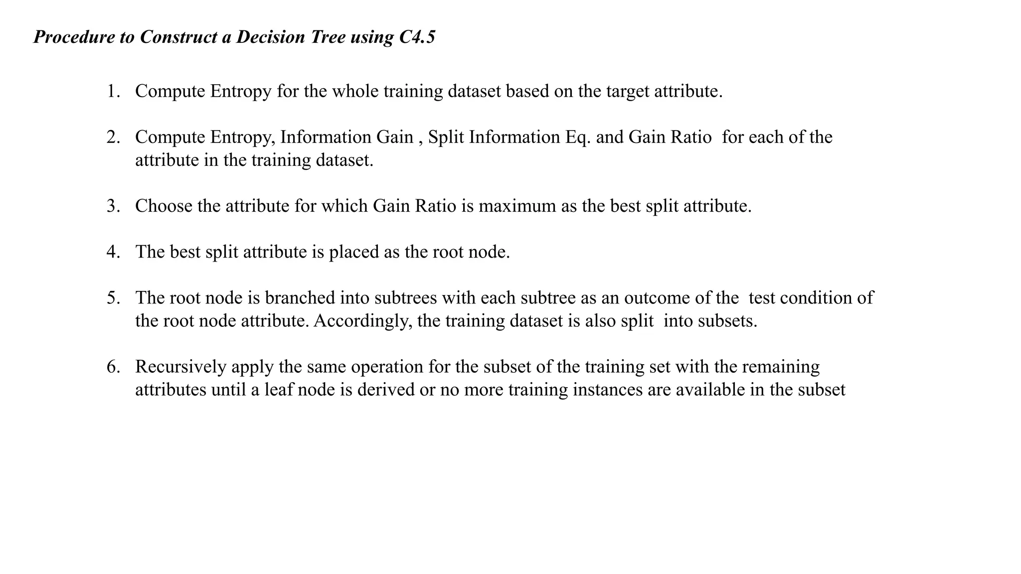
Procedure to Constructa Decision Tree using C4.5
1. Compute Entropy for the whole training dataset based on the target attribute.
2. Compute Entropy, Information Gain , Split Information Eq. and Gain Ratio for each of the
attribute in the training dataset.
3. Choose the attribute for which Gain Ratio is maximum as the best split attribute.
4. The best split attribute is placed as the root node.
5. The root node is branched into subtrees with each subtree as an outcome of the test condition of
the root node attribute. Accordingly, the training dataset is also split into subsets.
6. Recursively apply the same operation for the subset of the training set with the remaining
attributes until a leaf node is derived or no more training instances are available in the subset
45.
Entropy(S) = – pi log2 pi =
c
i=1
1. Compute Entropy
2. Information Gain
Gain(S, A) = Entropy(S) − Entropy(Sv)
|Sv|
|S|
v Values(A)
Values(A) possible values for A
Sv subset of S for which A has value v
4. Gain Ratio
SplitInfo(S, A) = − * log2
v Values(A)
|Sv|
|S|
|Sv|
|S|
3. Split Information
GainRatio(A) =
Gain(S, A)
SplitInfo(S, A)
46.
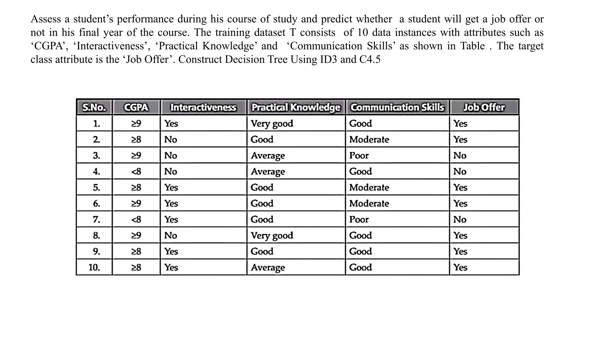
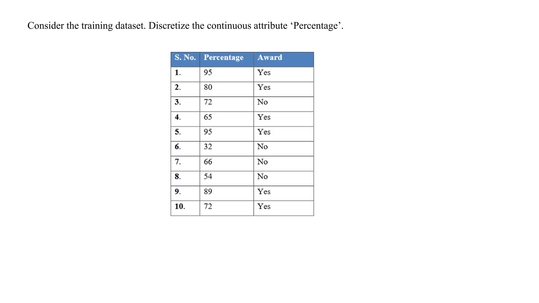
Assess a student’sperformance during his course of study and predict whether a student will get a job offer or
not in his final year of the course. The training dataset T consists of 10 data instances with attributes such as
‘CGPA’, ‘Interactiveness’, ‘Practical Knowledge’ and ‘Communication Skills’ as shown in Table . The target
class attribute is the ‘Job Offer’. Construct Decision Tree Using ID3 and C4.5
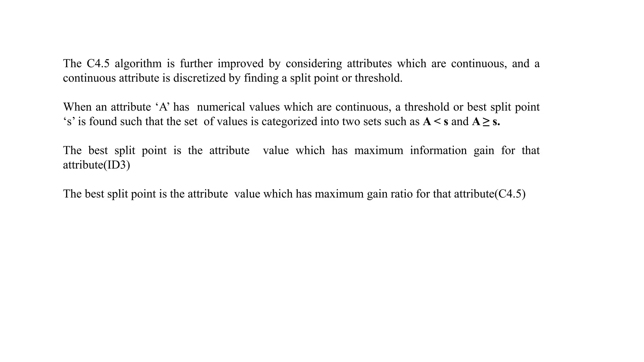
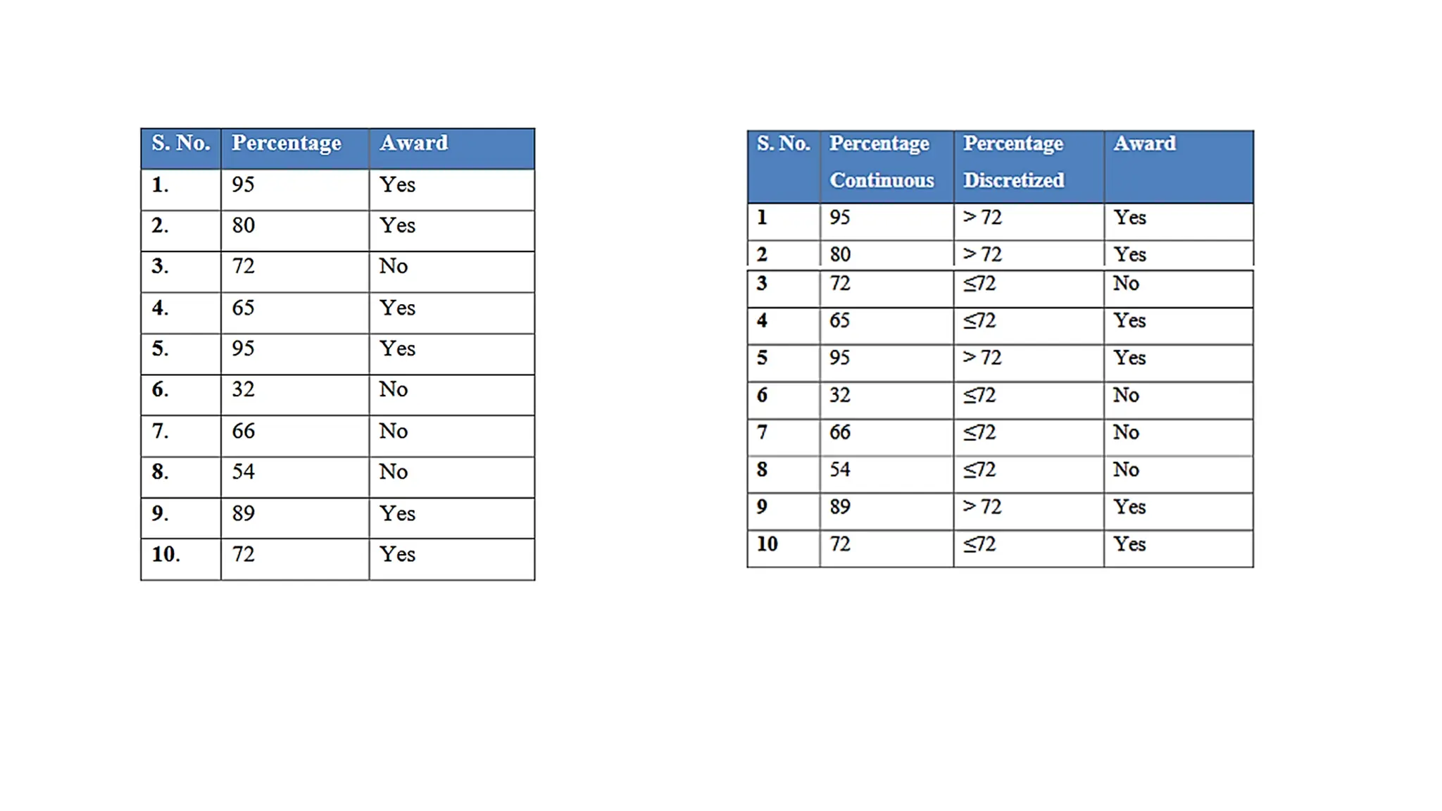
The C4.5 algorithmis further improved by considering attributes which are continuous, and a
continuous attribute is discretized by finding a split point or threshold.
When an attribute ‘A’ has numerical values which are continuous, a threshold or best split point
‘s’ is found such that the set of values is categorized into two sets such as A < s and A ≥ s.
The best split point is the attribute value which has maximum information gain for that
attribute(ID3)
The best split point is the attribute value which has maximum gain ratio for that attribute(C4.5)
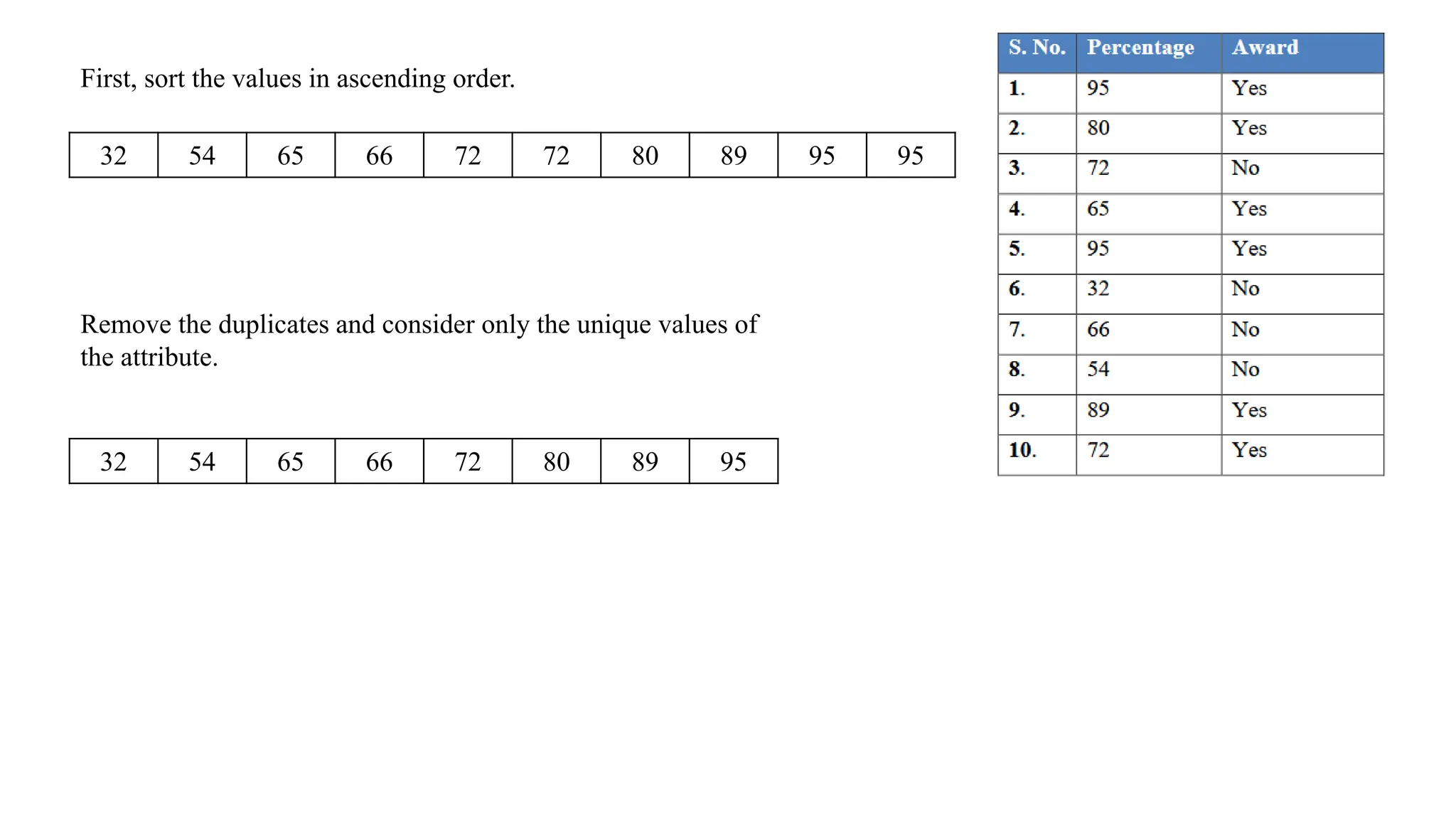
First, sort thevalues in ascending order.
32 54 65 66 72 72 80 89 95 95
Remove the duplicates and consider only the unique values of
the attribute.
32 54 65 66 72 80 89 95
51.
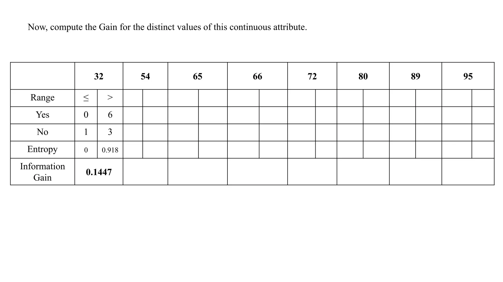
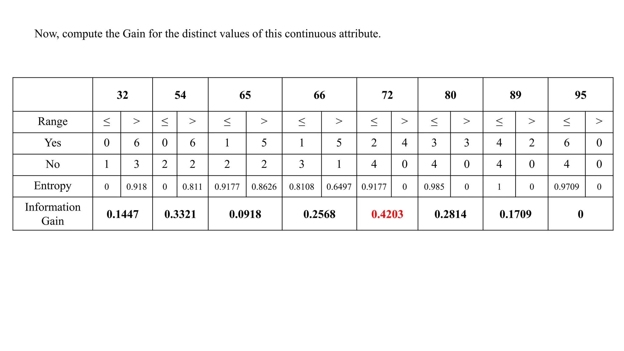
Now, compute theGain for the distinct values of this continuous attribute.
32 54 65 66 72 80 89 95
Range ≤ >
Yes 0 6
No 1 3
Entropy 0 0.918
Information
Gain
0.1447
The Classification andRegression Trees (CART) algorithm is a multivariate decision tree learning used for
classifying both categorical and continuous-valued target variables.
CART algorithm is an example of multivariate decision trees that gives oblique splits.
It solves both classification and regression problems.
If the target feature is categorical, it constructs a classification tree
if the target feature is continuous, it constructs a regression tree.
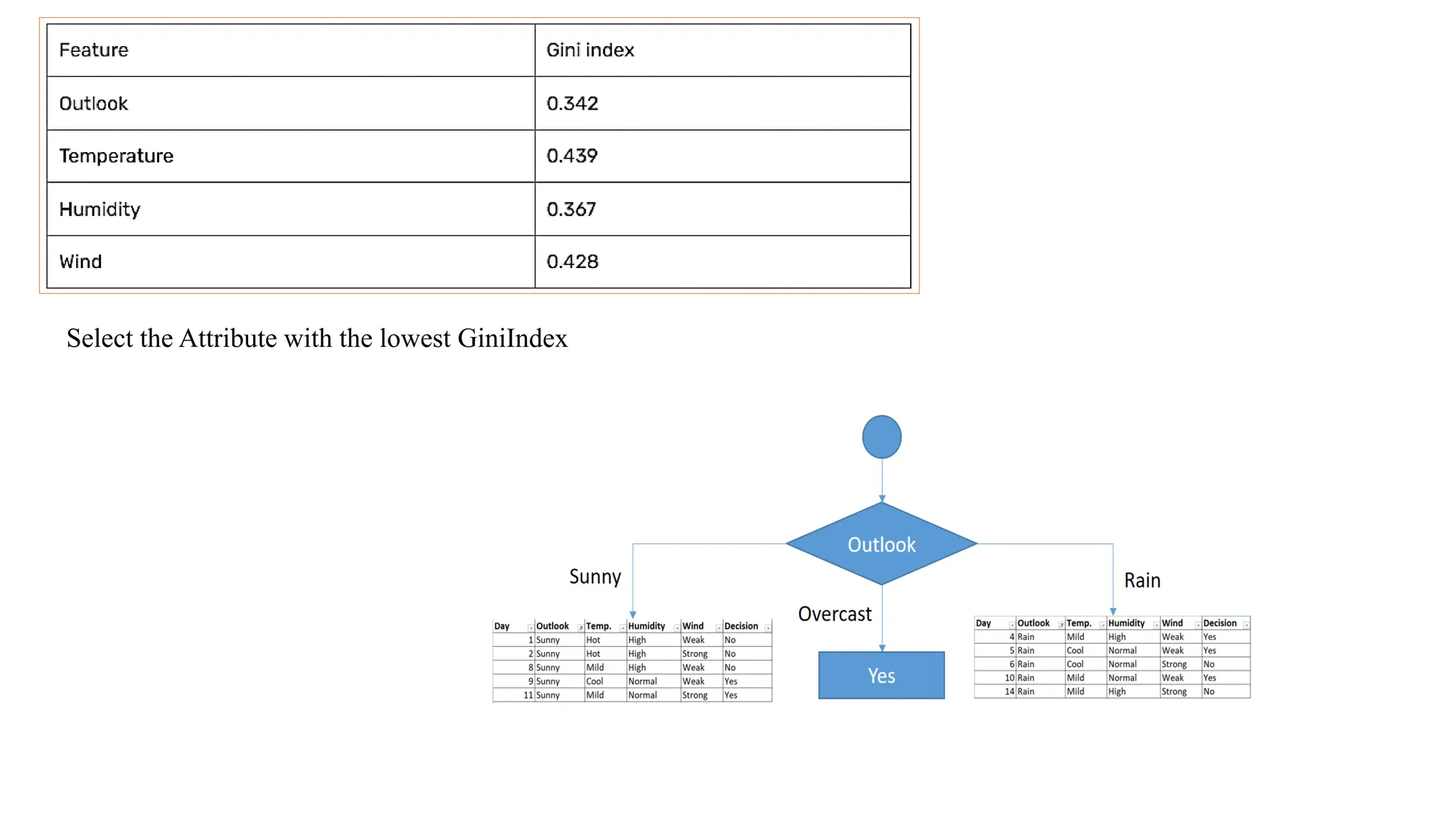
CART uses GINI Index to construct a decision tree.
GINI Index is defined as the number of data instances for a class or it is the proportion of instances.
It constructs the tree as a binary tree by recursively splitting a node into two nodes.
Therefore, even if an attribute has more than two possible values, GINI Index is calculated for all subsets of the
attributes and the subset which has maximum value is selected as the best split subset.
56.
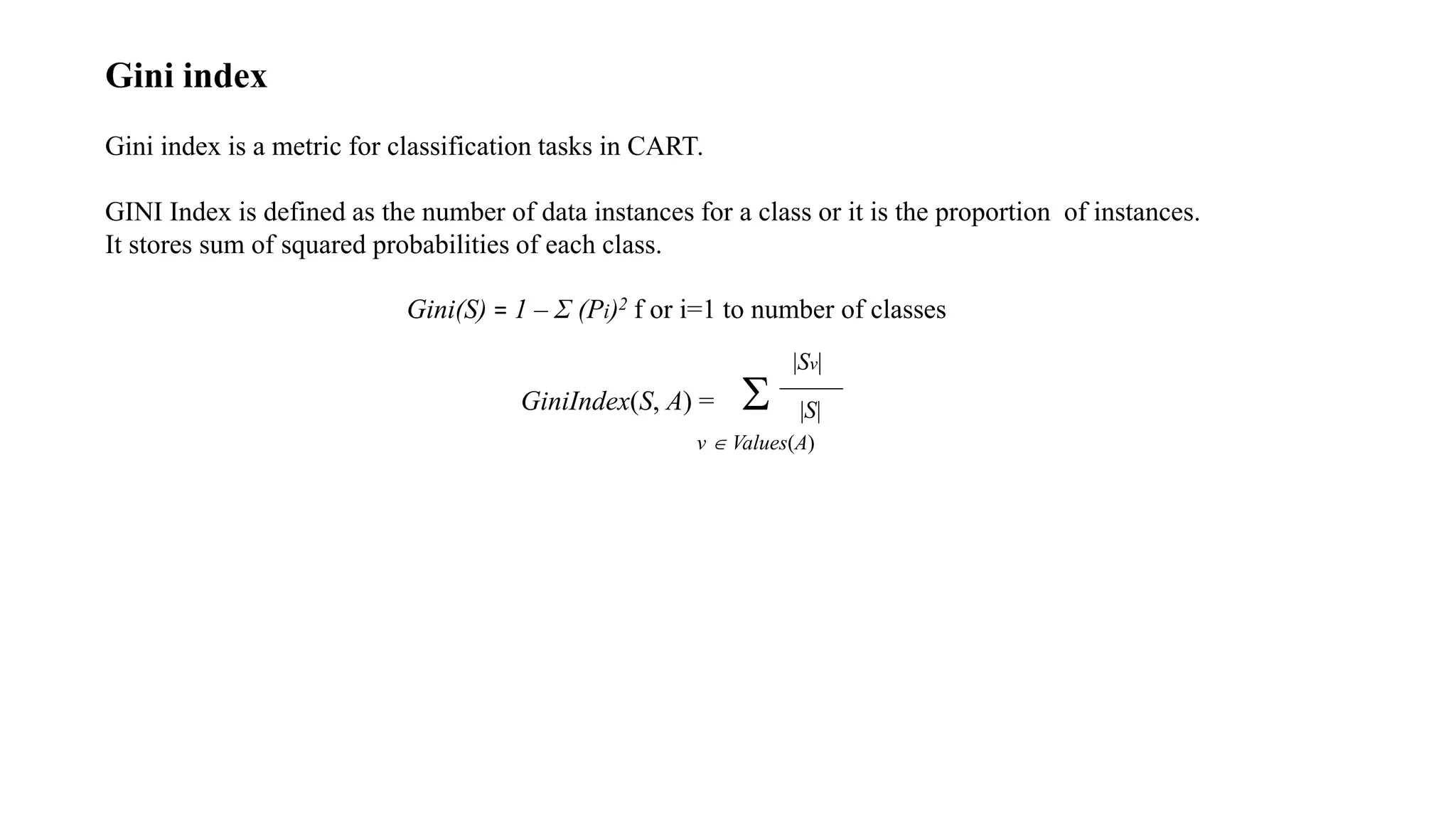
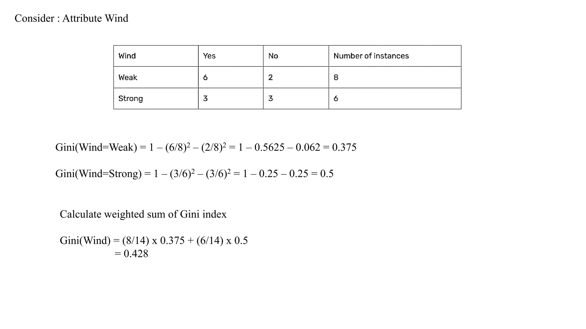
Gini index
Gini indexis a metric for classification tasks in CART.
GINI Index is defined as the number of data instances for a class or it is the proportion of instances.
It stores sum of squared probabilities of each class.
Gini(S) = 1 – Σ (Pi)2 f or i=1 to number of classes
GiniIndex(S, A) =
v Values(A)
|Sv|
|S|
57.
Problem 1:
Day OutlookTemperature Humidity Windy Play Tennis
D1 Sunny Hot High Weak No
D2 Sunny Hot High Strong No
D3 Overcast Hot High Weak Yes
D4 Rainy Mild High Weak Yes
D5 Rainy Cool Normal Weak Yes
D6 Rainy Cool Normal Strong No
D7 Overcast Cool Normal Strong Yes
D8 Sunny Mild High Weak No
D9 Sunny Cool Normal Weak Yes
D10 Rainy Mild Normal Weak Yes
D11 Sunny Mild Normal Strong Yes
D12 Overcast Mild High Strong Yes
D13 Overcast Hot Normal Weak Yes
D14 Rainy Mild High Strong No
Regression trees area variant of decision trees where the target feature is a continuous valued variable.
These trees can be constructed using an algorithm called reduction in variance which uses standard deviation to
choose the best splitting attribute.
Decision rules will be found based on standard deviations.
Procedure for Constructing Regression Trees
1. Compute standard deviation for each attribute with respect to target attribute.
2. Compute standard deviation for the number of data instances of each distinct value of an attribute.
3. Compute weighted standard deviation for each attribute.
4. Compute standard deviation reduction by subtracting weighted standard deviation for each attribute from
standard deviation of each attribute.
5. Choose the attribute with a higher standard deviation reduction as the best split attribute.
6. The best split attribute is placed as the root node.
7. The root node is branched into subtrees with each subtree as an outcome of the test condition of the root
node attribute. Accordingly, the training dataset is also split into different subsets.
8. Recursively apply the same operation for the subset of the training set with the remaining attributes until a
leaf node is derived or no more training instances are available in the subset.
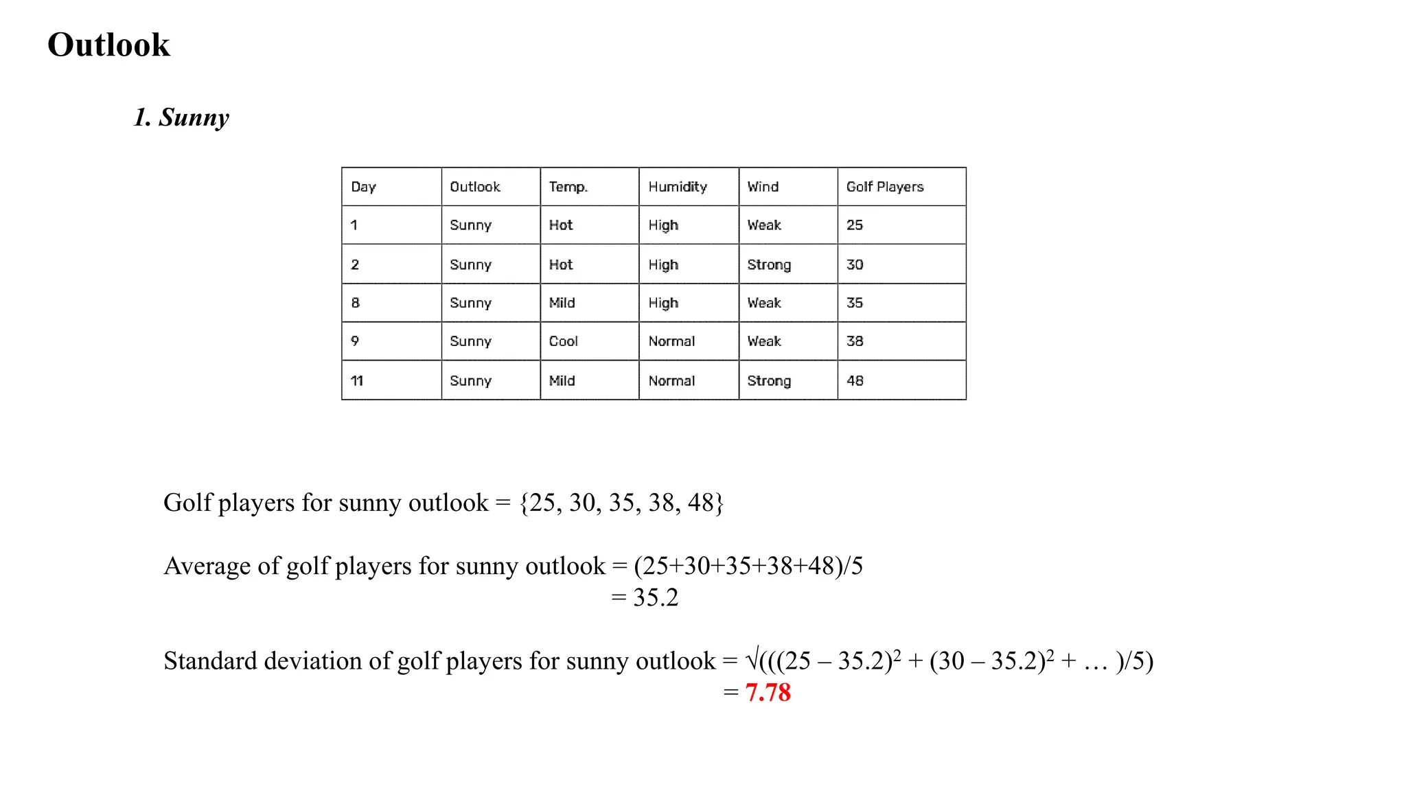
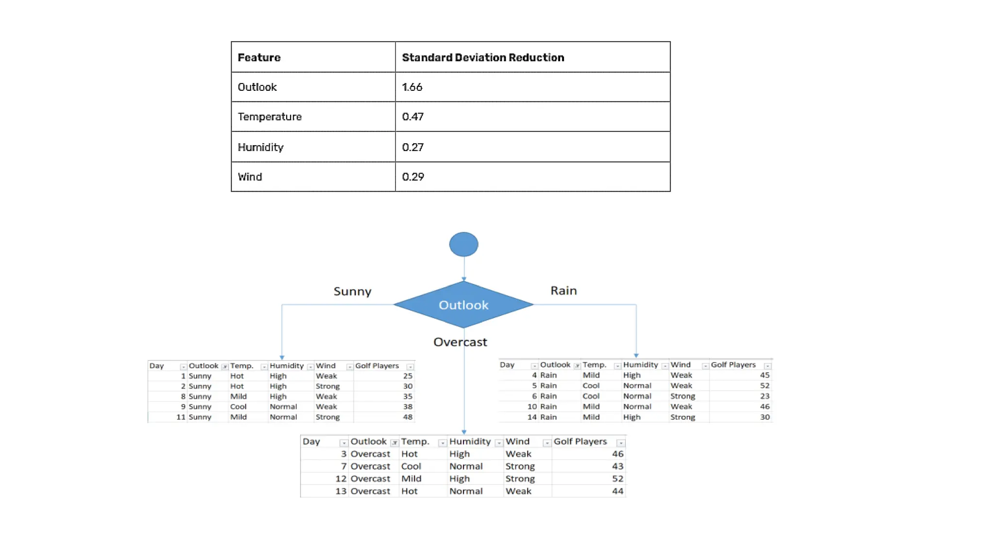
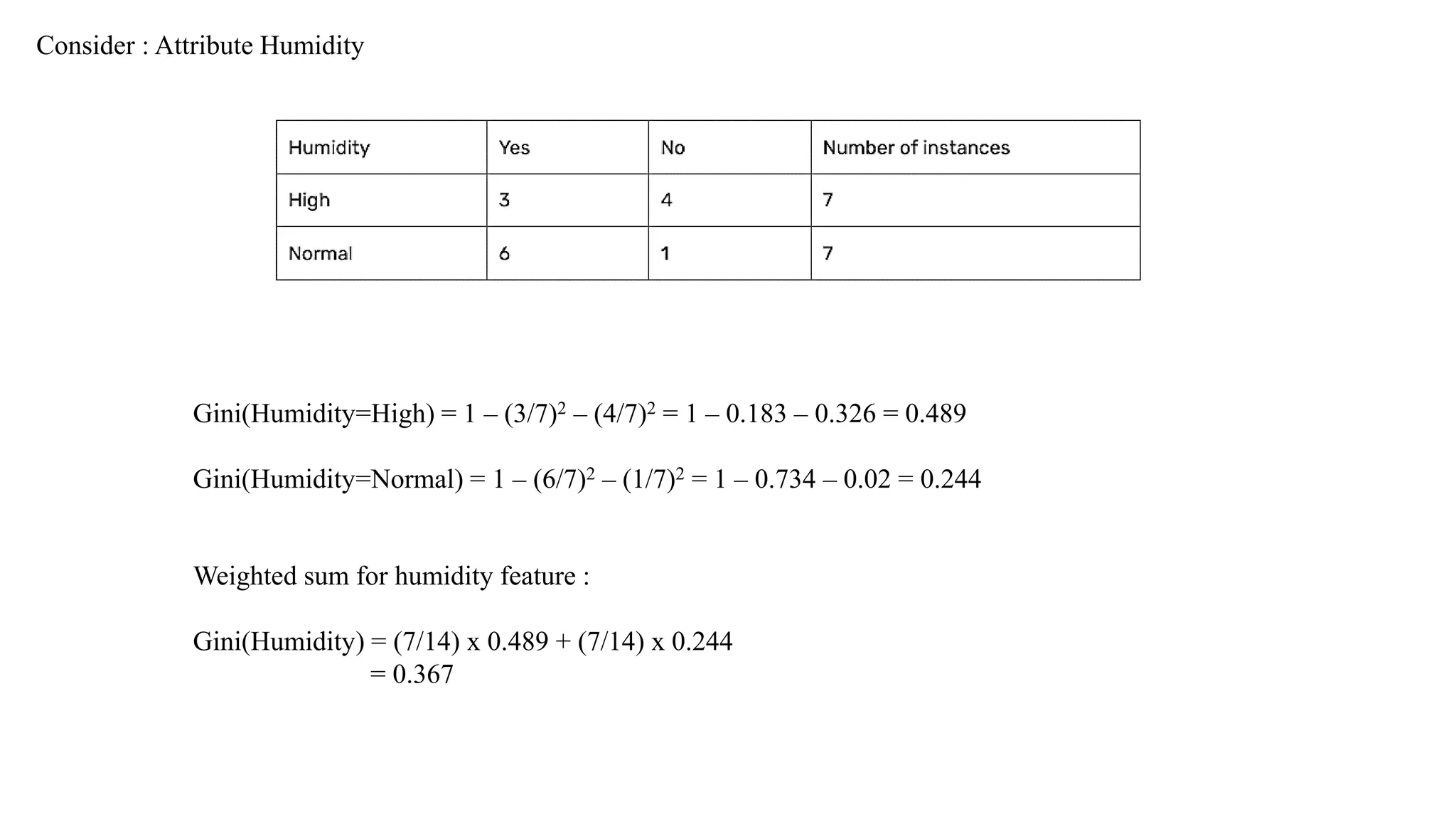
Outlook
1. Sunny
Golf playersfor sunny outlook = {25, 30, 35, 38, 48}
Average of golf players for sunny outlook = (25+30+35+38+48)/5
= 35.2
Standard deviation of golf players for sunny outlook = √(((25 – 35.2)2 + (30 – 35.2)2 + … )/5)
= 7.78
78.
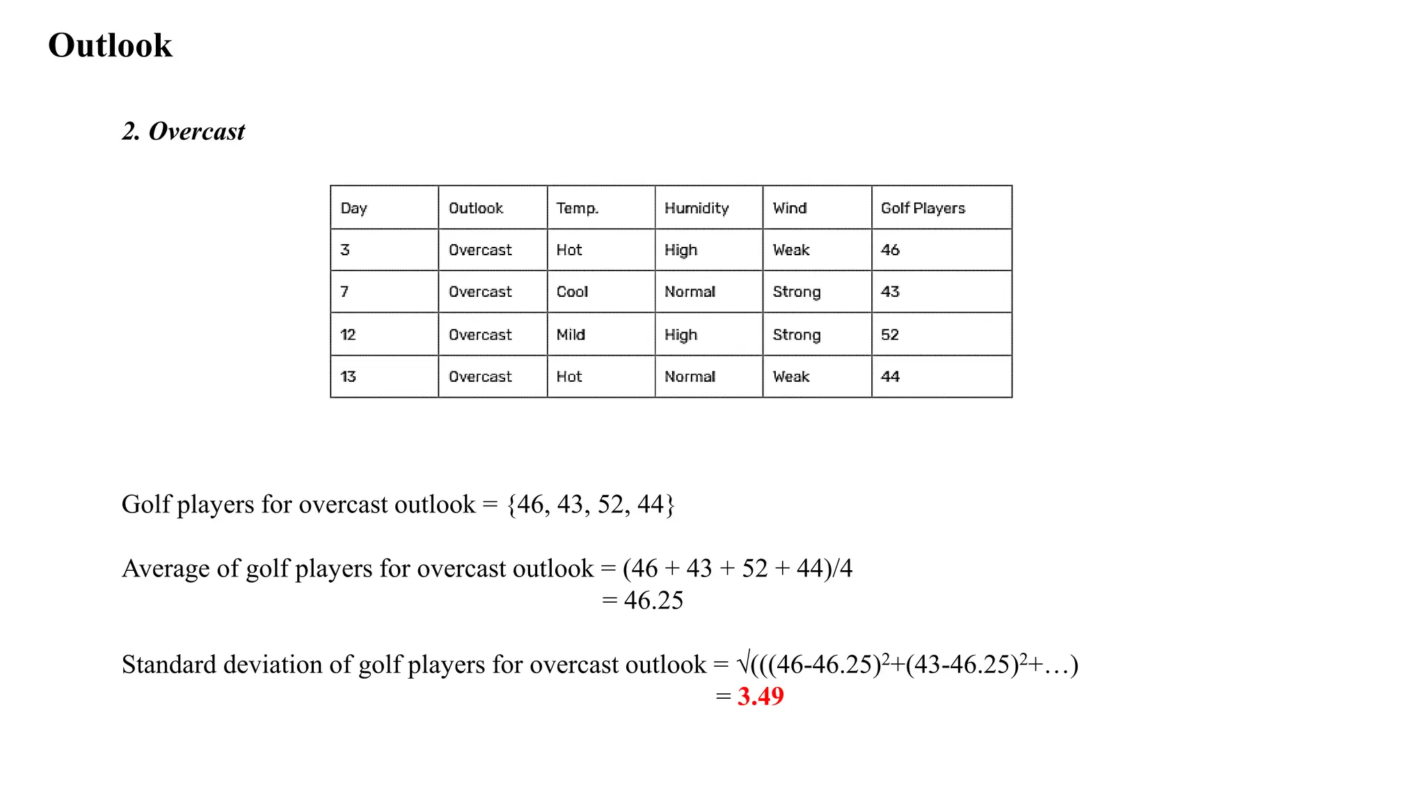
Outlook
2. Overcast
Golf playersfor overcast outlook = {46, 43, 52, 44}
Average of golf players for overcast outlook = (46 + 43 + 52 + 44)/4
= 46.25
Standard deviation of golf players for overcast outlook = √(((46-46.25)2+(43-46.25)2+…)
= 3.49
79.
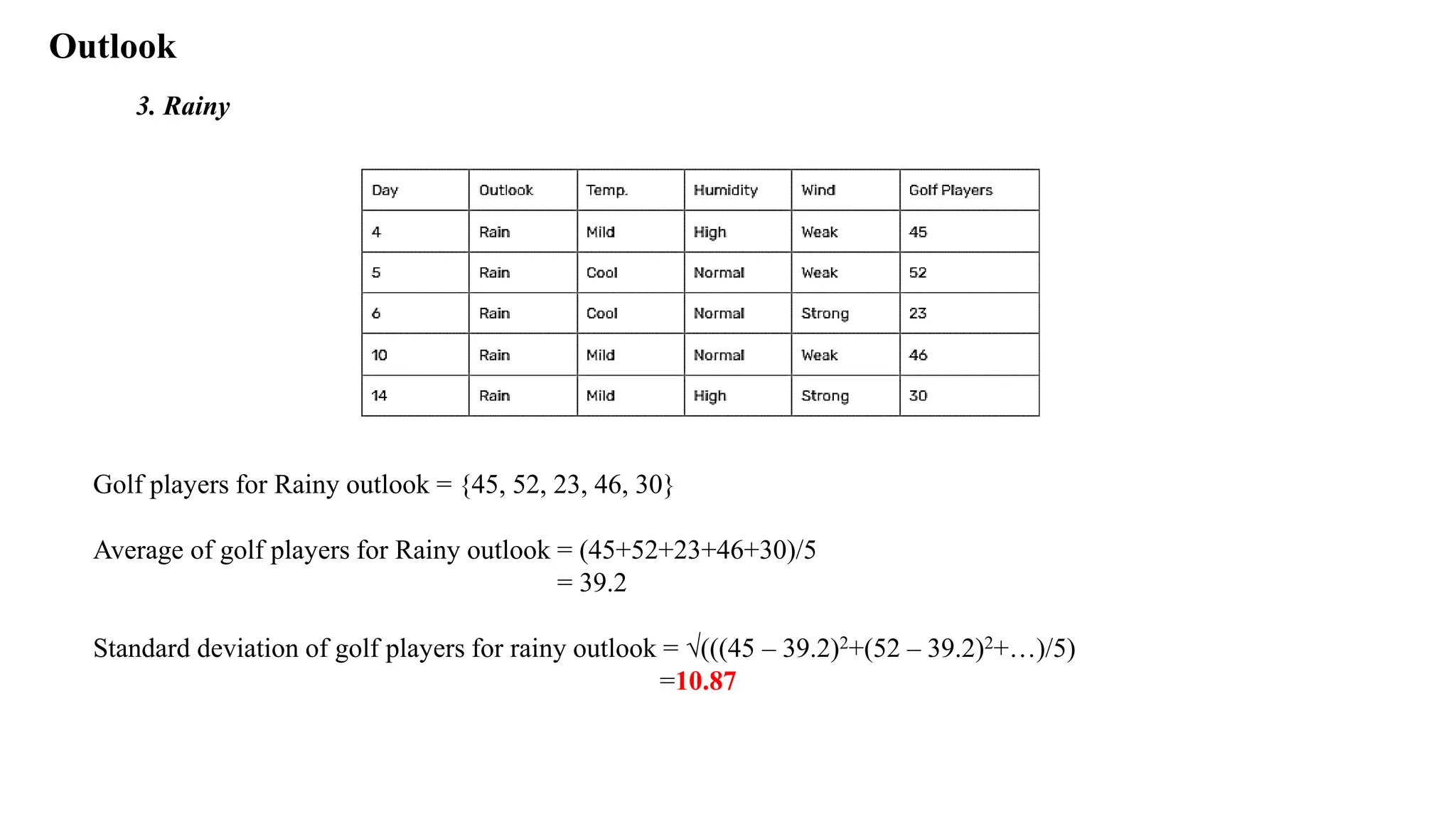
Outlook
3. Rainy
Golf playersfor Rainy outlook = {45, 52, 23, 46, 30}
Average of golf players for Rainy outlook = (45+52+23+46+30)/5
= 39.2
Standard deviation of golf players for rainy outlook = √(((45 – 39.2)2+(52 – 39.2)2+…)/5)
=10.87
80.
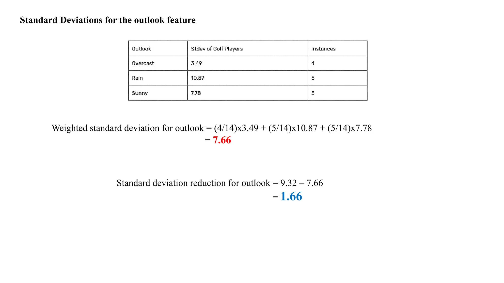
Standard Deviations forthe outlook feature
Weighted standard deviation for outlook = (4/14)x3.49 + (5/14)x10.87 + (5/14)x7.78
= 7.66
Standard deviation reduction for outlook = 9.32 – 7.66
= 1.66
81.
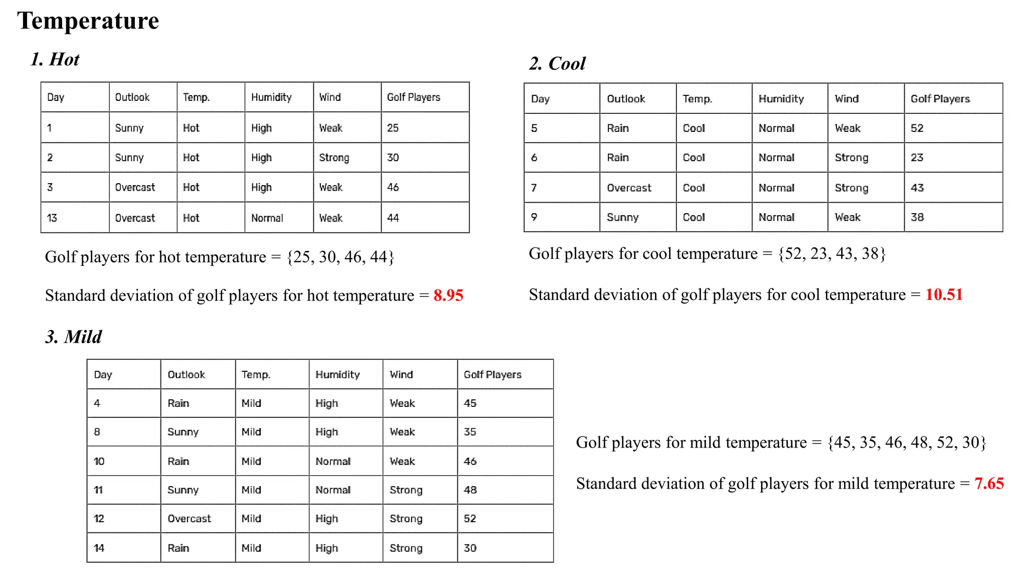
Temperature
1. Hot 2.Cool
Golf players for hot temperature = {25, 30, 46, 44}
Standard deviation of golf players for hot temperature = 8.95
Golf players for cool temperature = {52, 23, 43, 38}
Standard deviation of golf players for cool temperature = 10.51
3. Mild
Golf players for mild temperature = {45, 35, 46, 48, 52, 30}
Standard deviation of golf players for mild temperature = 7.65
82.
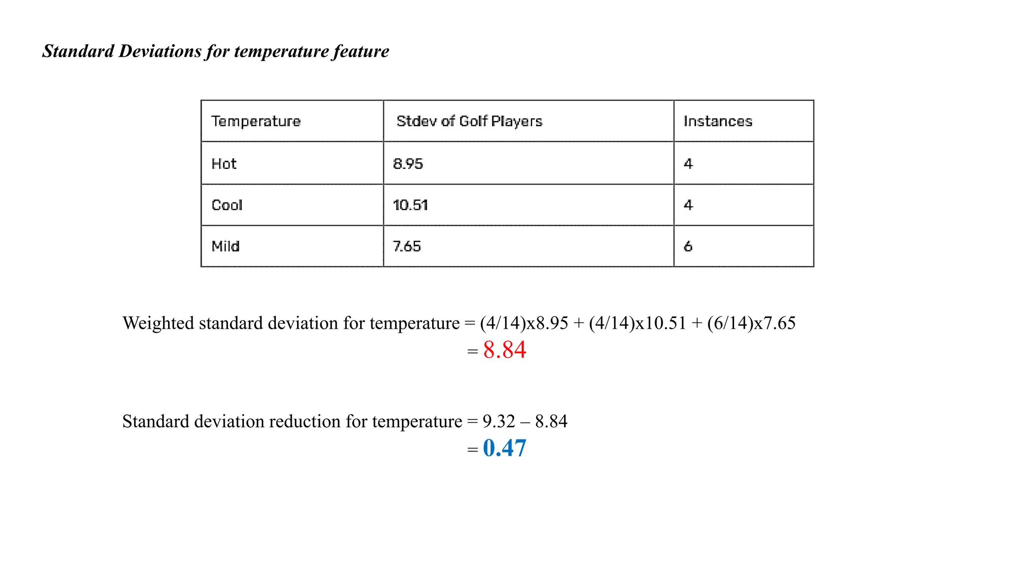
Standard Deviations fortemperature feature
Weighted standard deviation for temperature = (4/14)x8.95 + (4/14)x10.51 + (6/14)x7.65
= 8.84
Standard deviation reduction for temperature = 9.32 – 8.84
= 0.47
83.
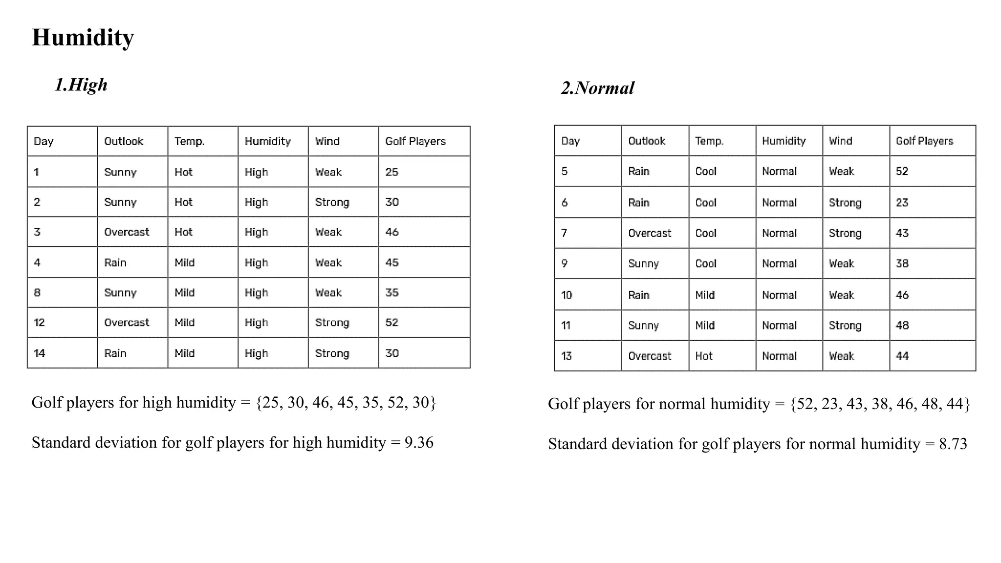
Humidity
1.High 2.Normal
Golf playersfor high humidity = {25, 30, 46, 45, 35, 52, 30}
Standard deviation for golf players for high humidity = 9.36
Golf players for normal humidity = {52, 23, 43, 38, 46, 48, 44}
Standard deviation for golf players for normal humidity = 8.73
84.
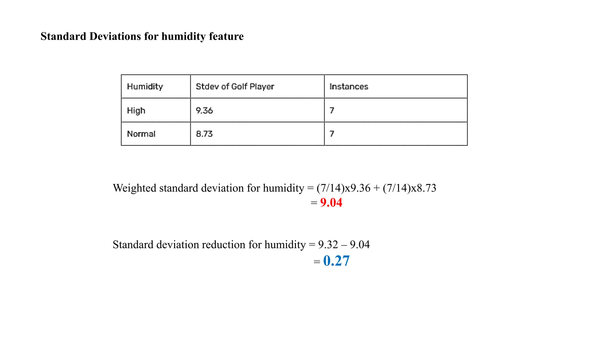
Standard Deviations forhumidity feature
Weighted standard deviation for humidity = (7/14)x9.36 + (7/14)x8.73
= 9.04
Standard deviation reduction for humidity = 9.32 – 9.04
= 0.27
85.
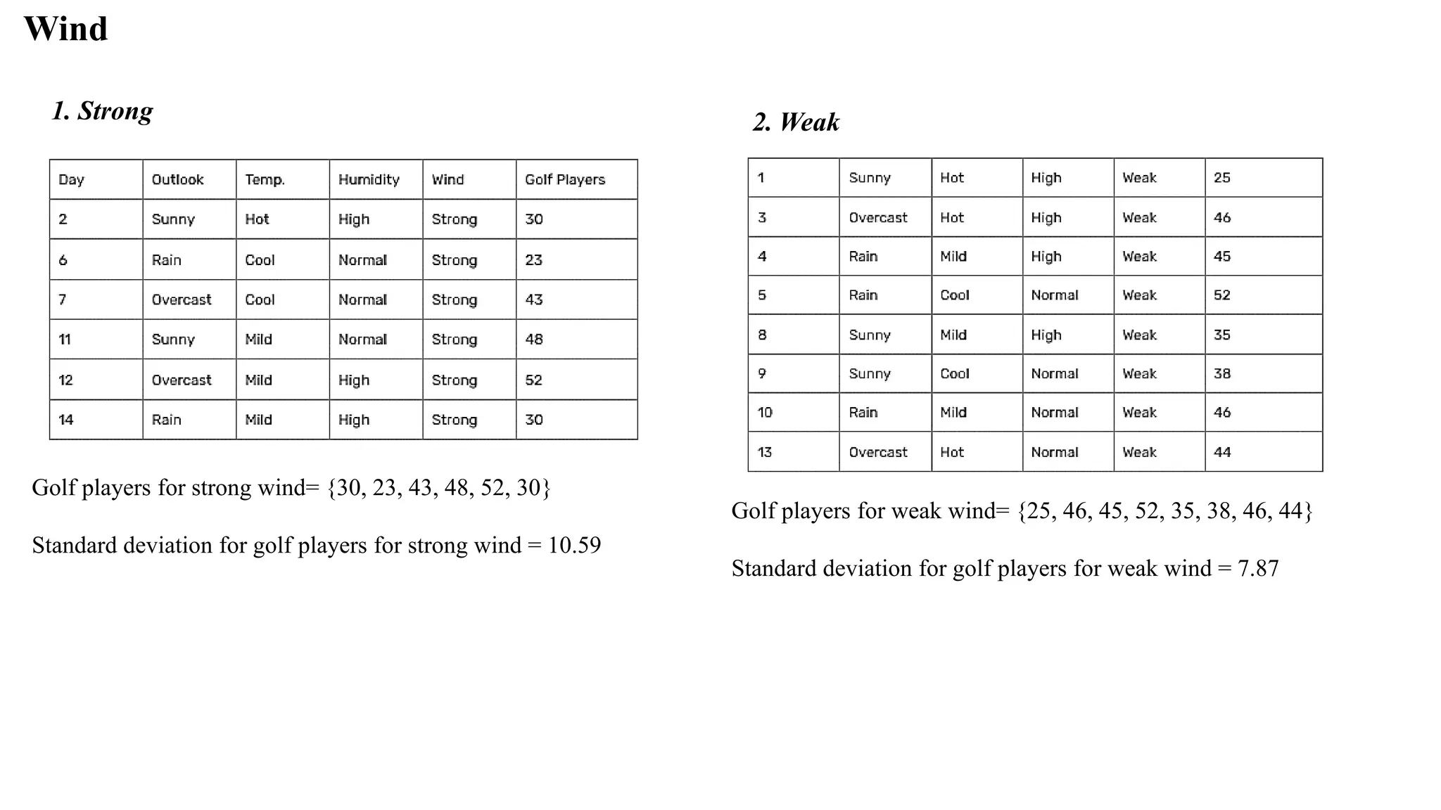
Wind
1. Strong 2.Weak
Golf players for weak wind= {25, 46, 45, 52, 35, 38, 46, 44}
Standard deviation for golf players for weak wind = 7.87
Golf players for strong wind= {30, 23, 43, 48, 52, 30}
Standard deviation for golf players for strong wind = 10.59
86.
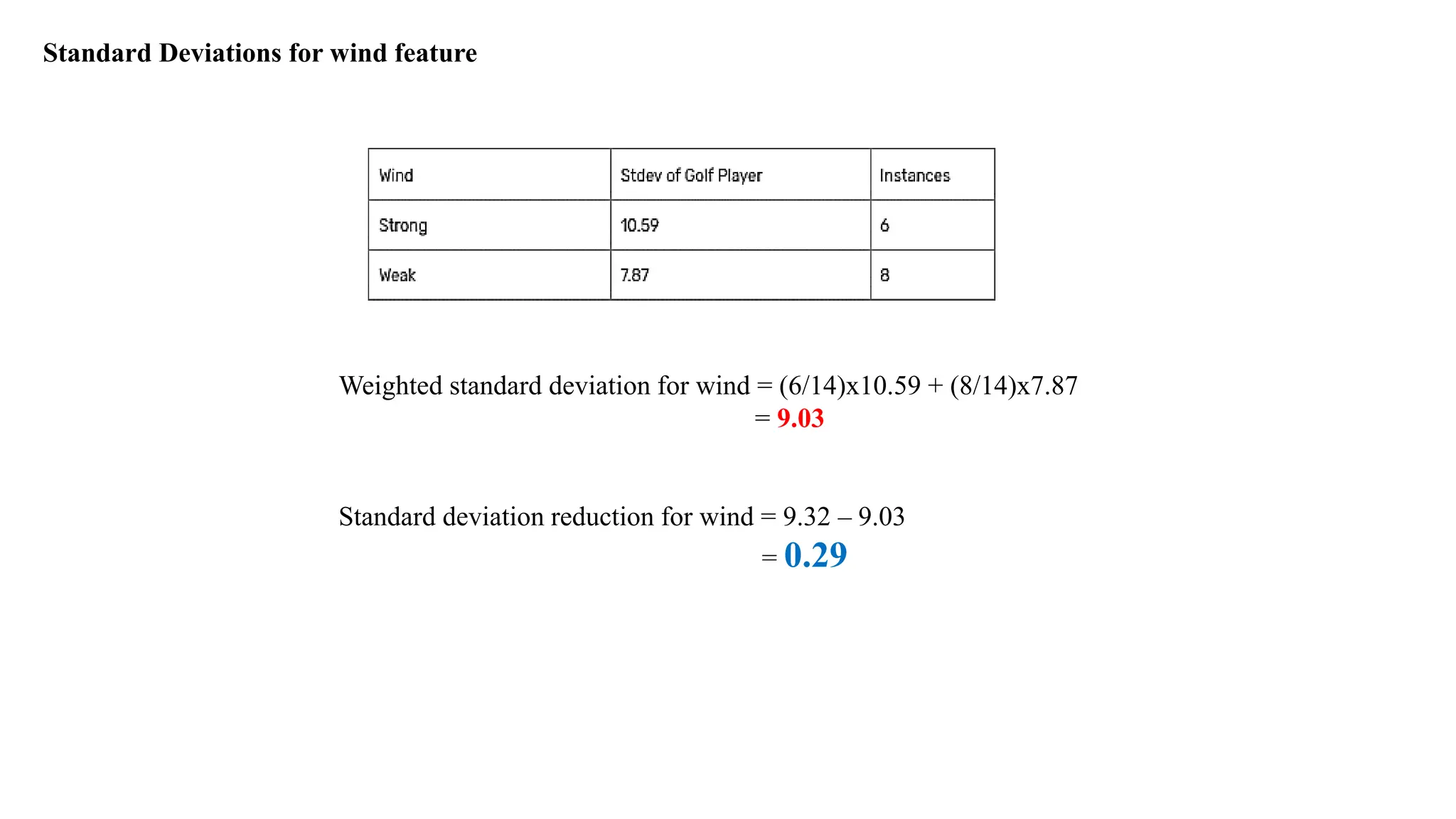
Standard Deviations forwind feature
Weighted standard deviation for wind = (6/14)x10.59 + (8/14)x7.87
= 9.03
Standard deviation reduction for wind = 9.32 – 9.03
= 0.29
88.
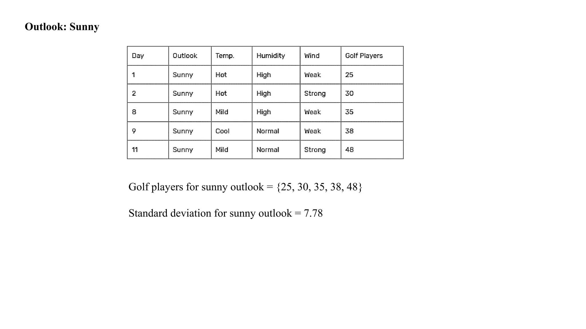
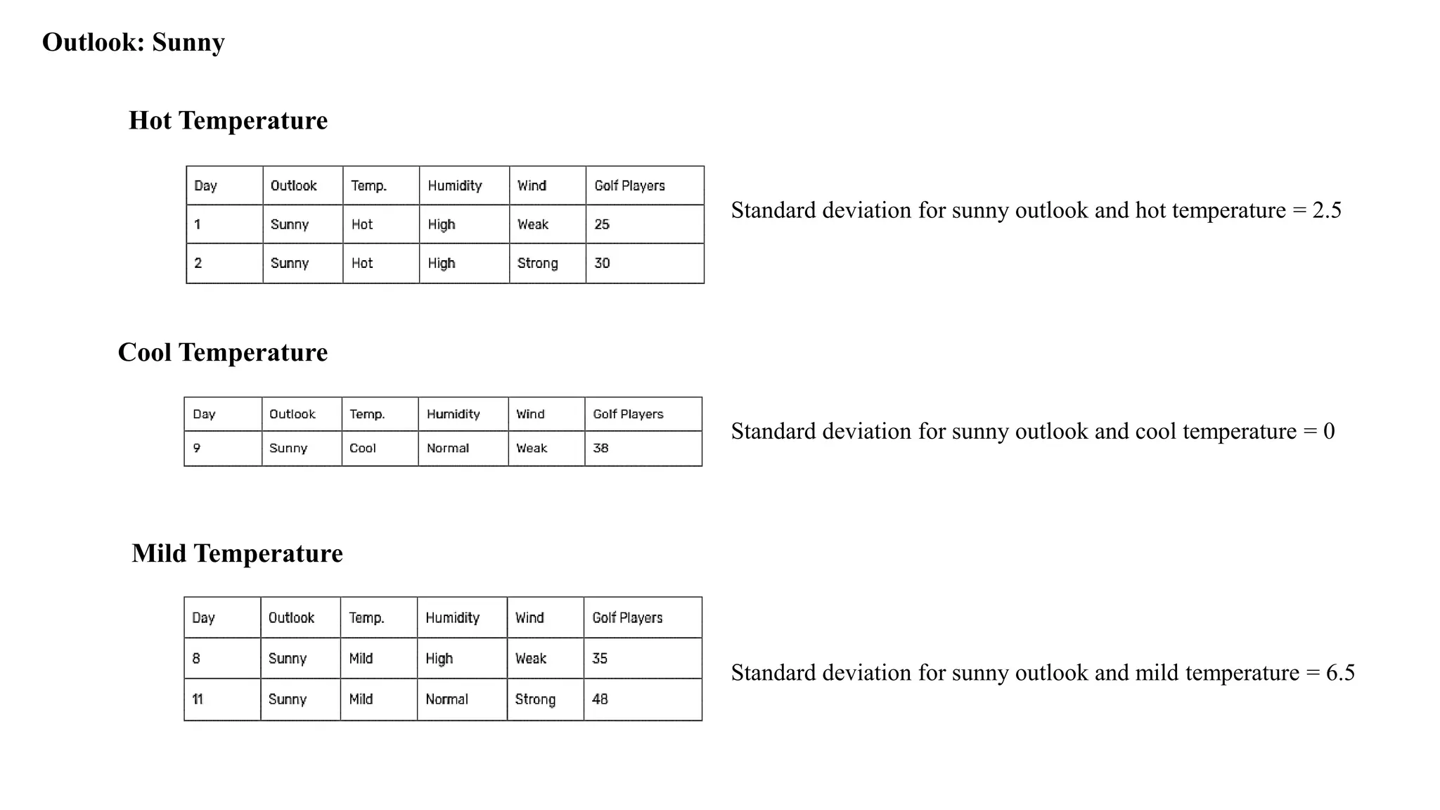
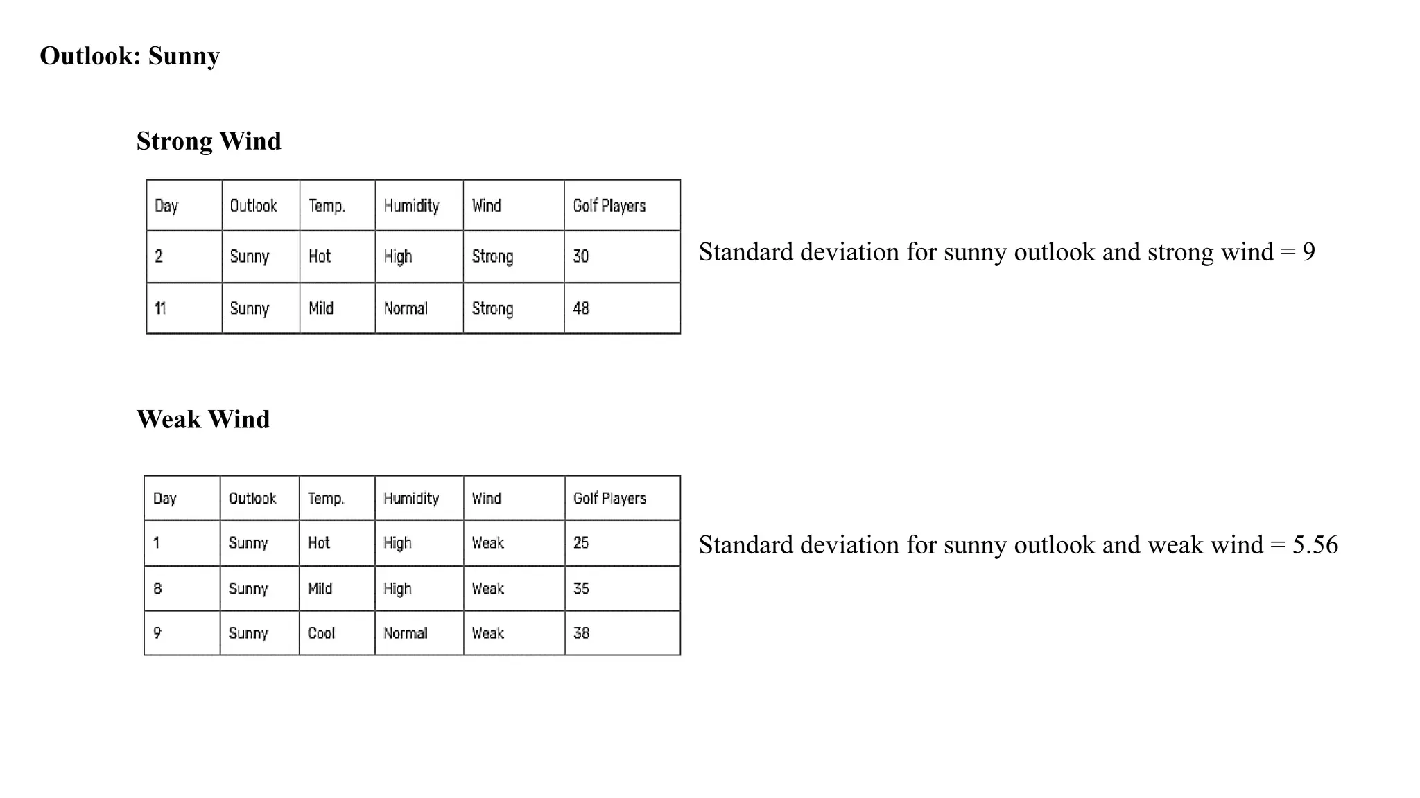
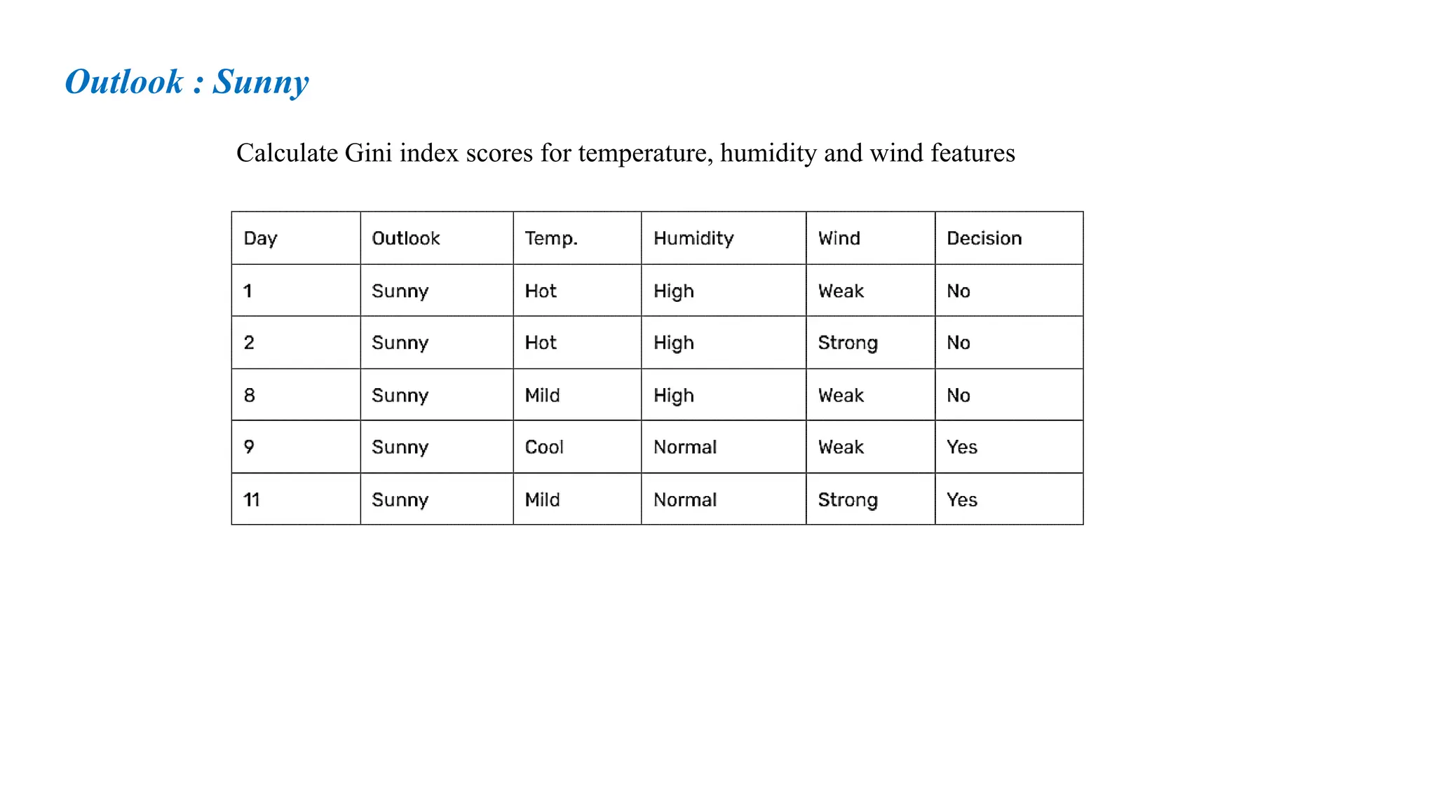
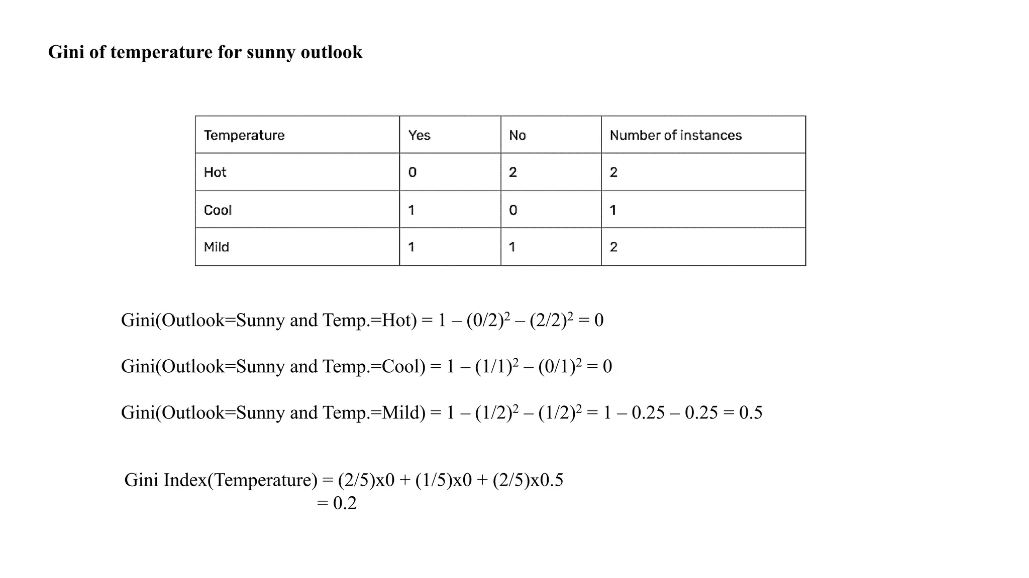
Outlook: Sunny
Golf playersfor sunny outlook = {25, 30, 35, 38, 48}
Standard deviation for sunny outlook = 7.78
89.
Outlook: Sunny
Hot Temperature
Standarddeviation for sunny outlook and hot temperature = 2.5
Cool Temperature
Standard deviation for sunny outlook and cool temperature = 0
Mild Temperature
Standard deviation for sunny outlook and mild temperature = 6.5
90.
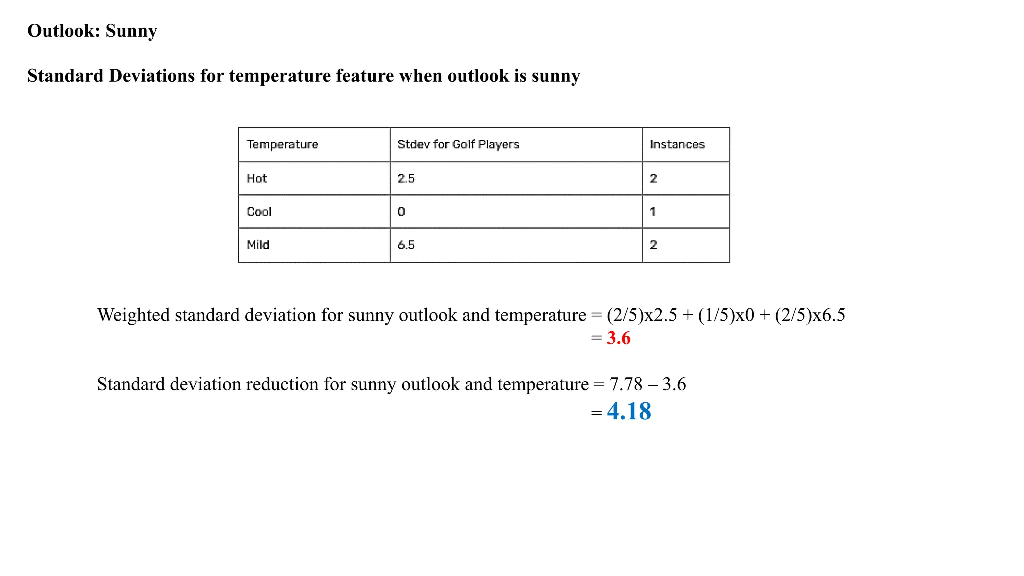
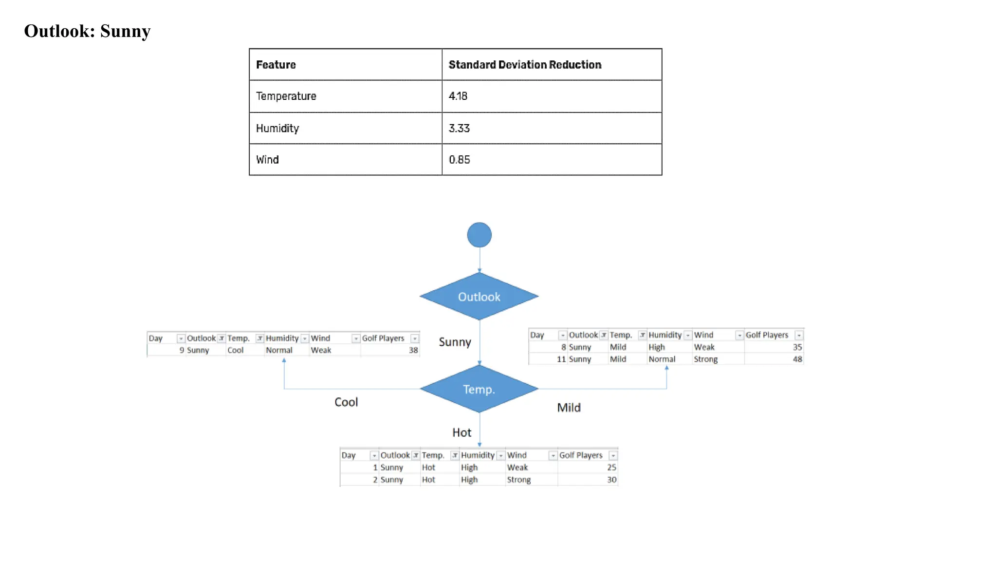
Standard Deviations fortemperature feature when outlook is sunny
Weighted standard deviation for sunny outlook and temperature = (2/5)x2.5 + (1/5)x0 + (2/5)x6.5
= 3.6
Standard deviation reduction for sunny outlook and temperature = 7.78 – 3.6
= 4.18
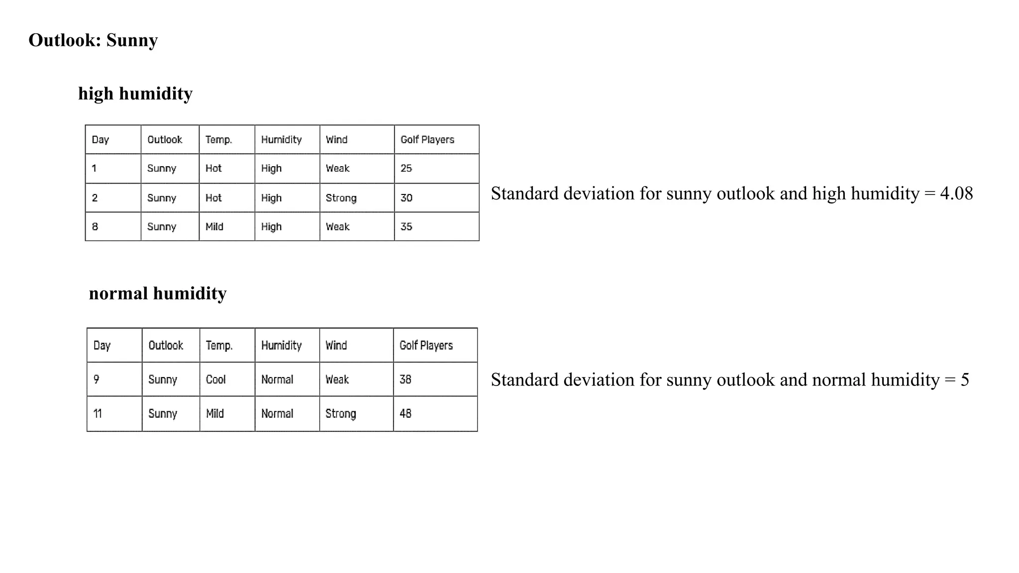
Outlook: Sunny
91.
high humidity
Standard deviationfor sunny outlook and high humidity = 4.08
normal humidity
Standard deviation for sunny outlook and normal humidity = 5
Outlook: Sunny
92.
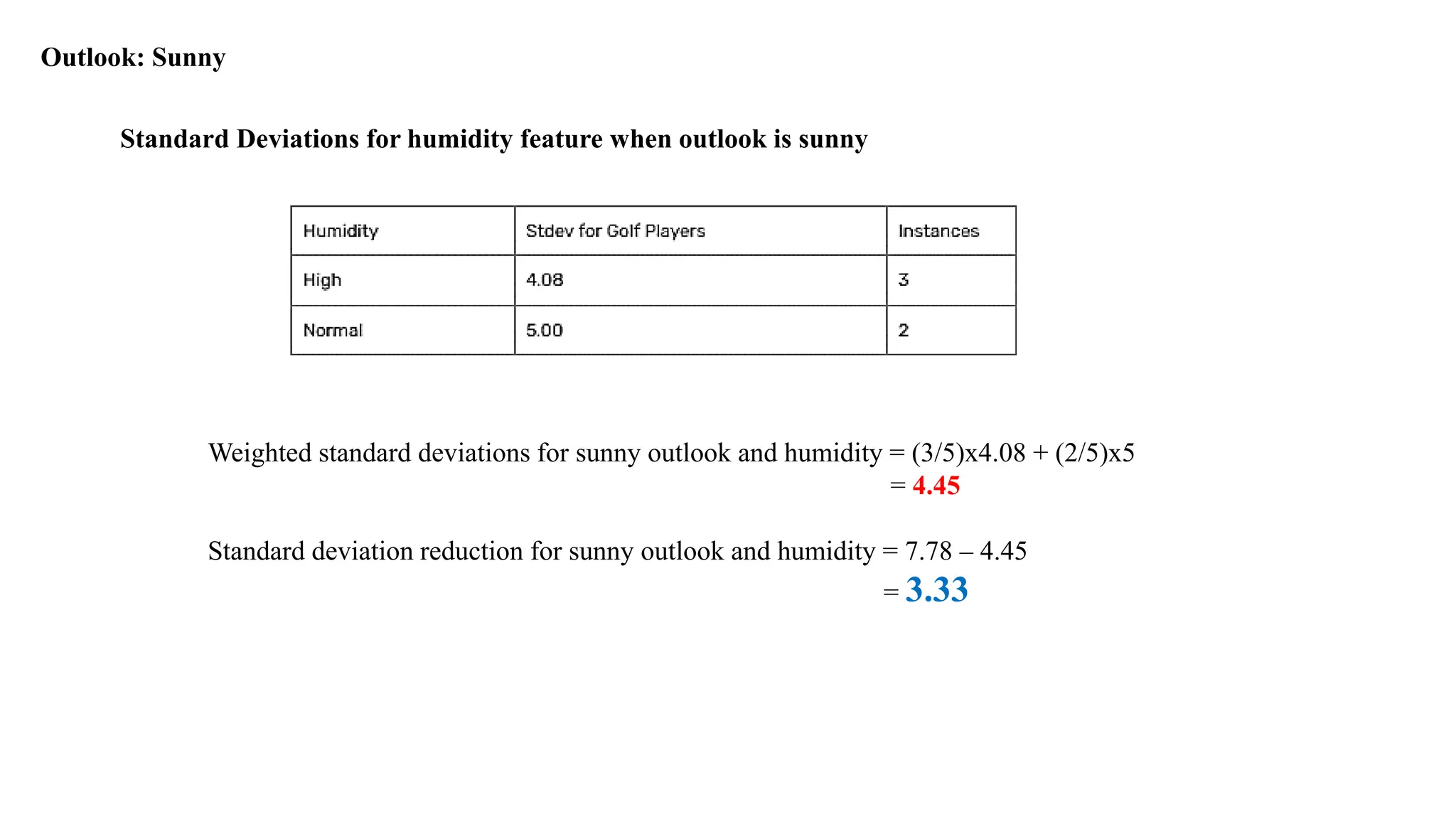
Standard Deviations forhumidity feature when outlook is sunny
Weighted standard deviations for sunny outlook and humidity = (3/5)x4.08 + (2/5)x5
= 4.45
Standard deviation reduction for sunny outlook and humidity = 7.78 – 4.45
= 3.33
Outlook: Sunny
93.
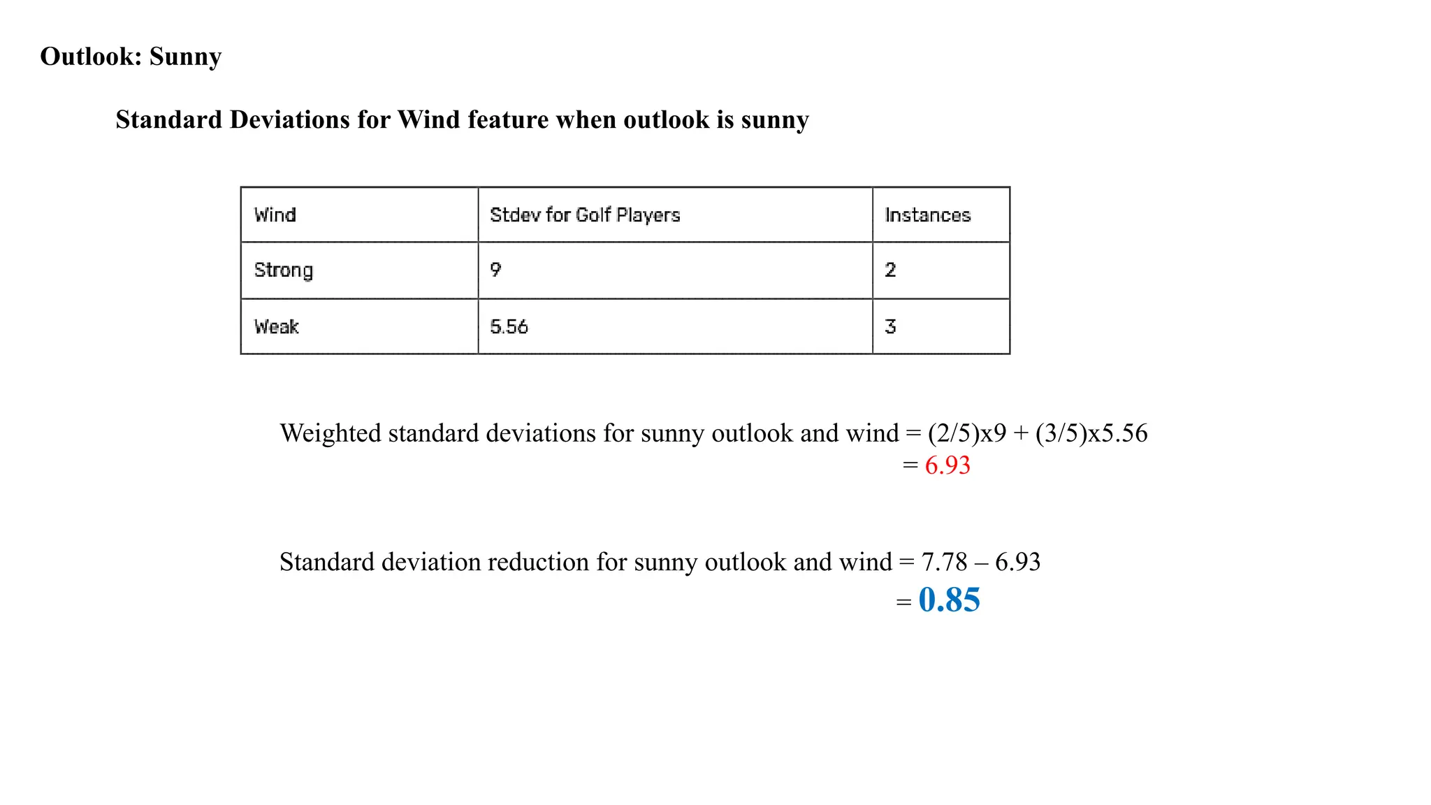
Strong Wind
Standard deviationfor sunny outlook and strong wind = 9
Weak Wind
Standard deviation for sunny outlook and weak wind = 5.56
Outlook: Sunny
94.
Weighted standard deviationsfor sunny outlook and wind = (2/5)x9 + (3/5)x5.56
= 6.93
Standard deviation reduction for sunny outlook and wind = 7.78 – 6.93
= 0.85
Standard Deviations for Wind feature when outlook is sunny
Outlook: Sunny
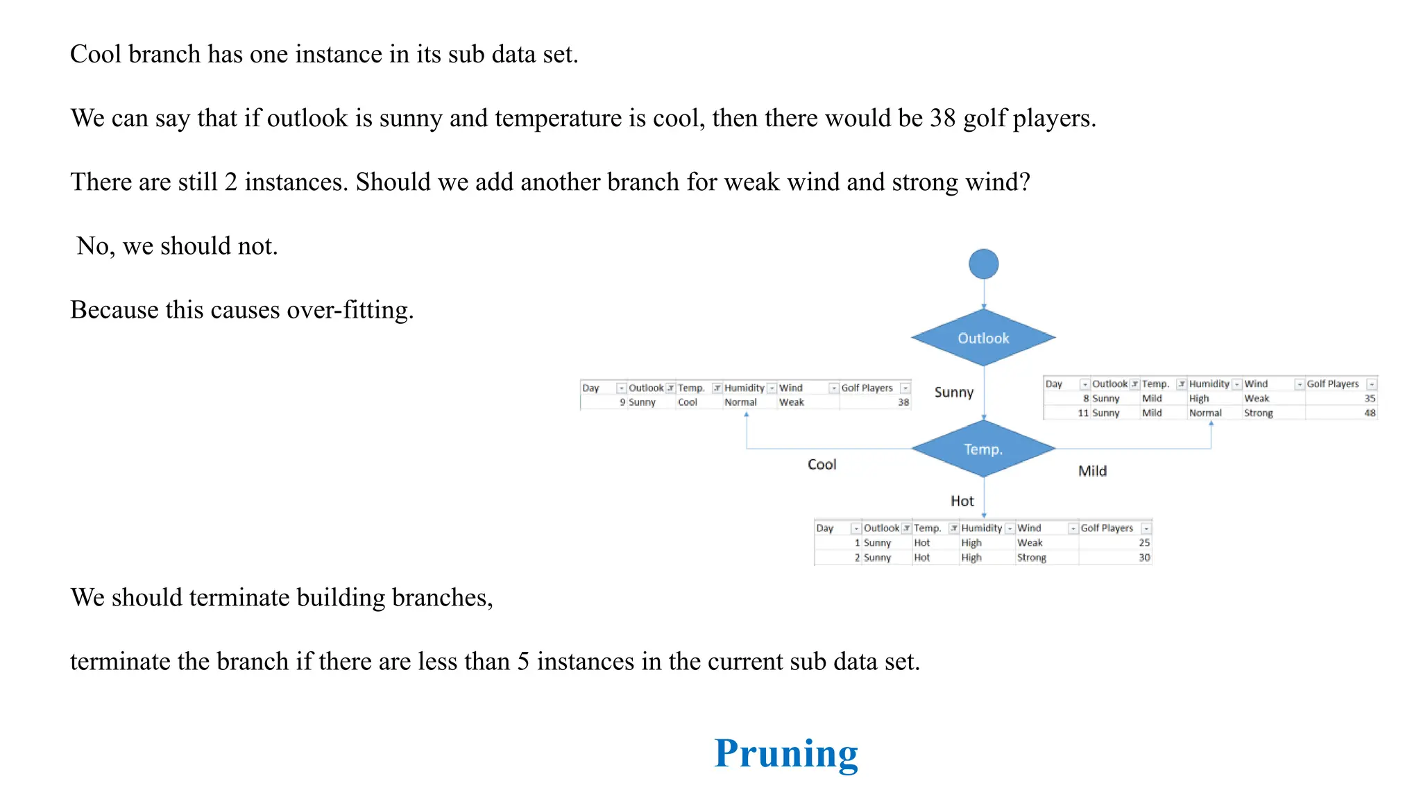
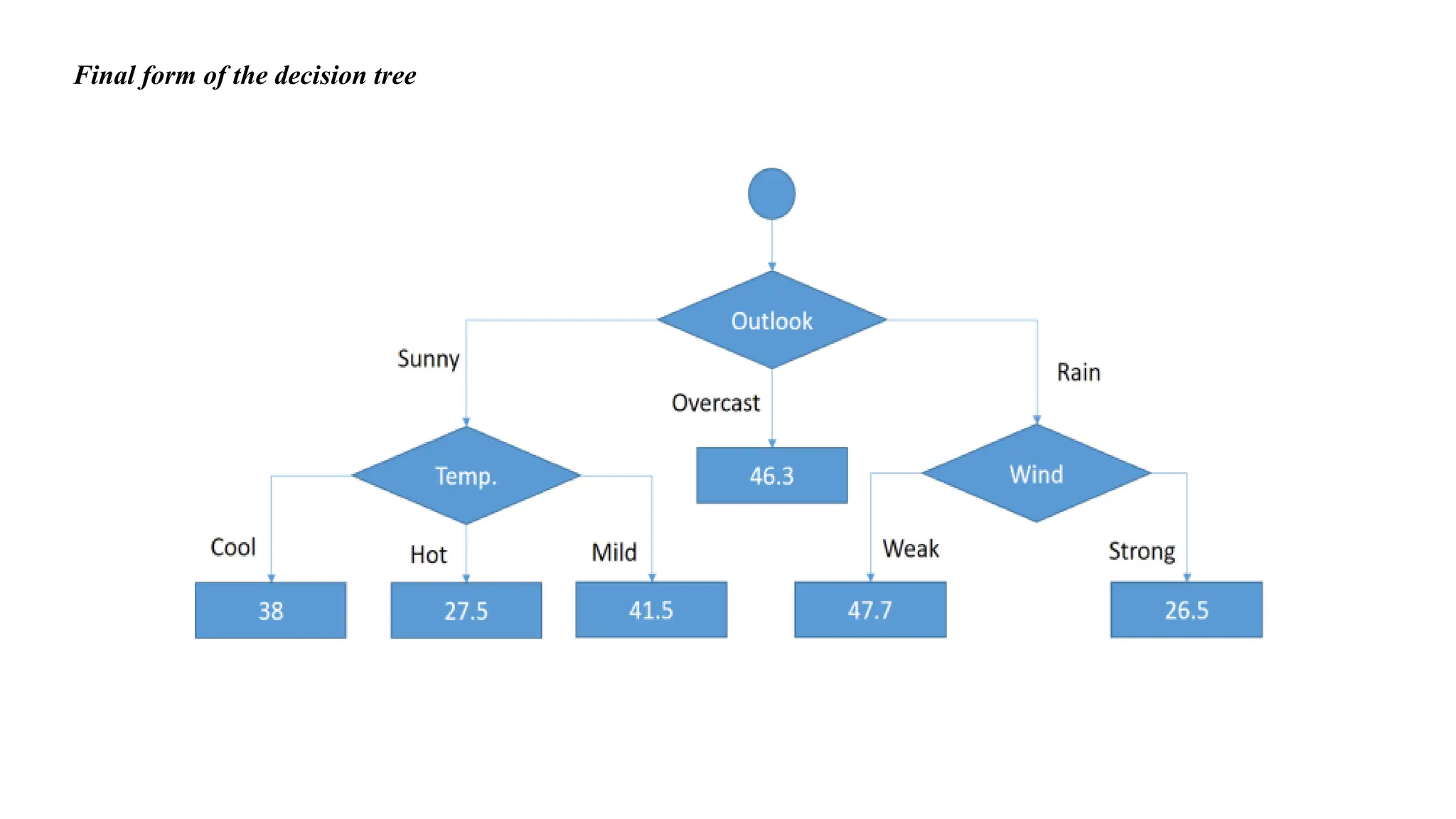
Cool branch hasone instance in its sub data set.
We can say that if outlook is sunny and temperature is cool, then there would be 38 golf players.
There are still 2 instances. Should we add another branch for weak wind and strong wind?
No, we should not.
Because this causes over-fitting.
We should terminate building branches,
terminate the branch if there are less than 5 instances in the current sub data set.
Pruning
97.
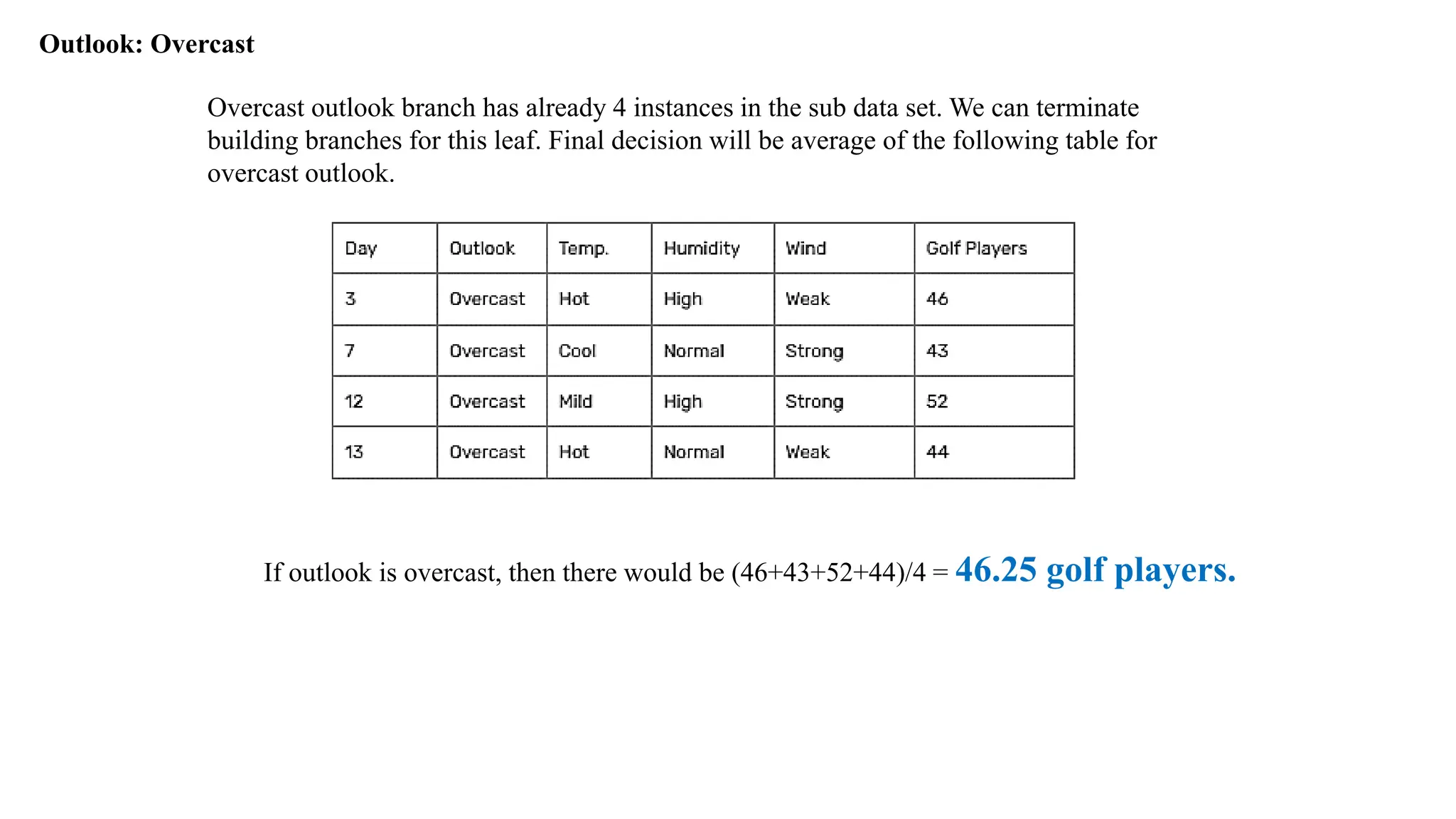
Outlook: Overcast
Overcast outlookbranch has already 4 instances in the sub data set. We can terminate
building branches for this leaf. Final decision will be average of the following table for
overcast outlook.
If outlook is overcast, then there would be (46+43+52+44)/4 = 46.25 golf players.
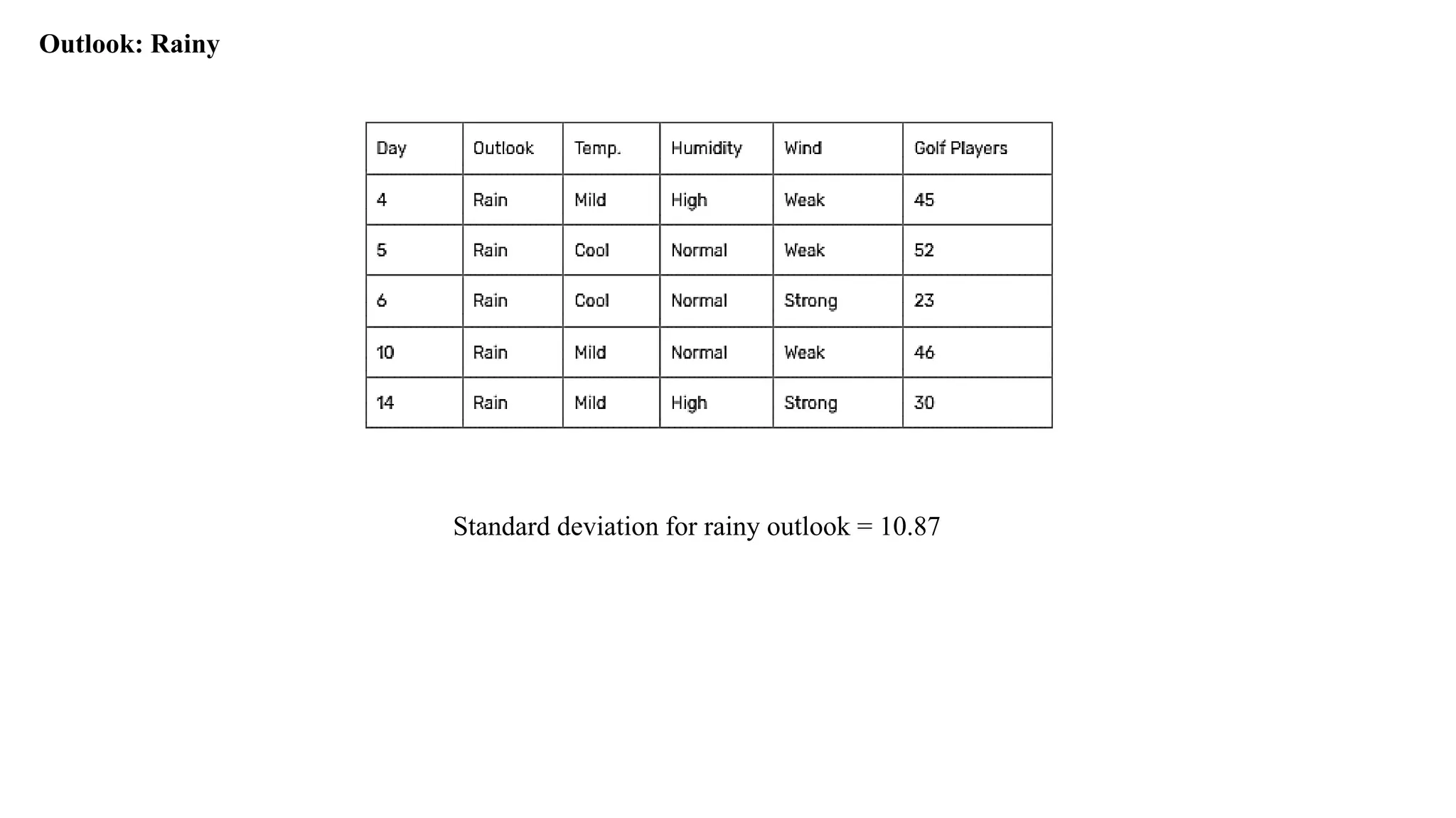
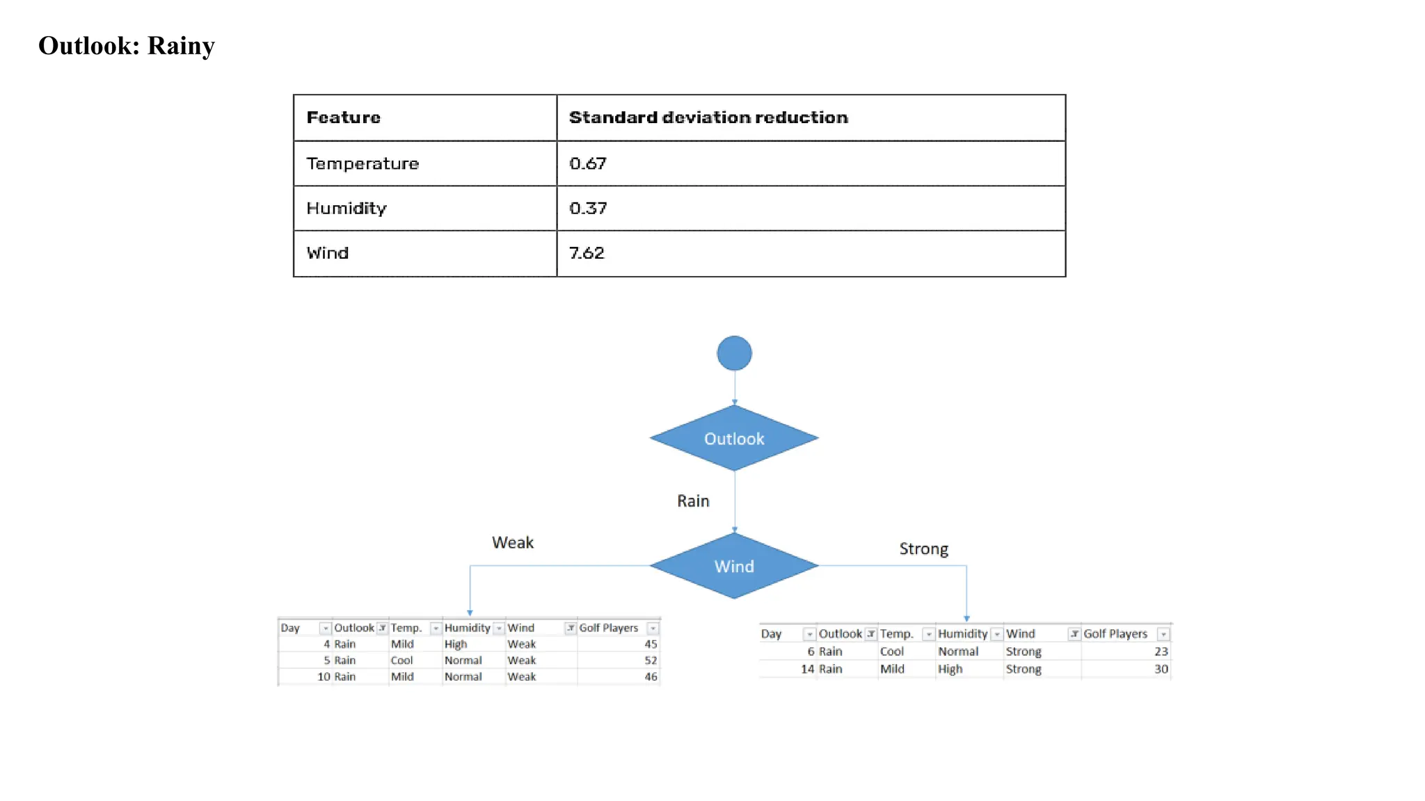
Outlook: Rainy
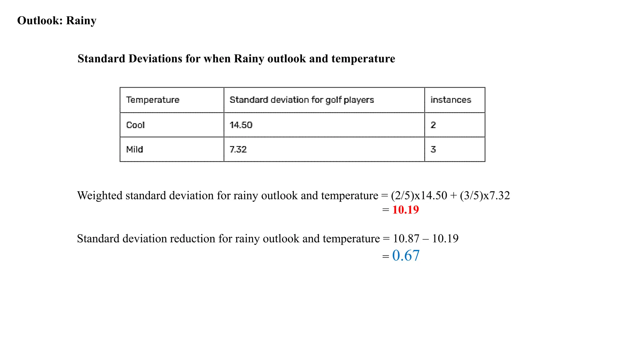
Standard Deviationsfor when Rainy outlook and temperature
Weighted standard deviation for rainy outlook and temperature = (2/5)x14.50 + (3/5)x7.32
= 10.19
Standard deviation reduction for rainy outlook and temperature = 10.87 – 10.19
= 0.67
100.
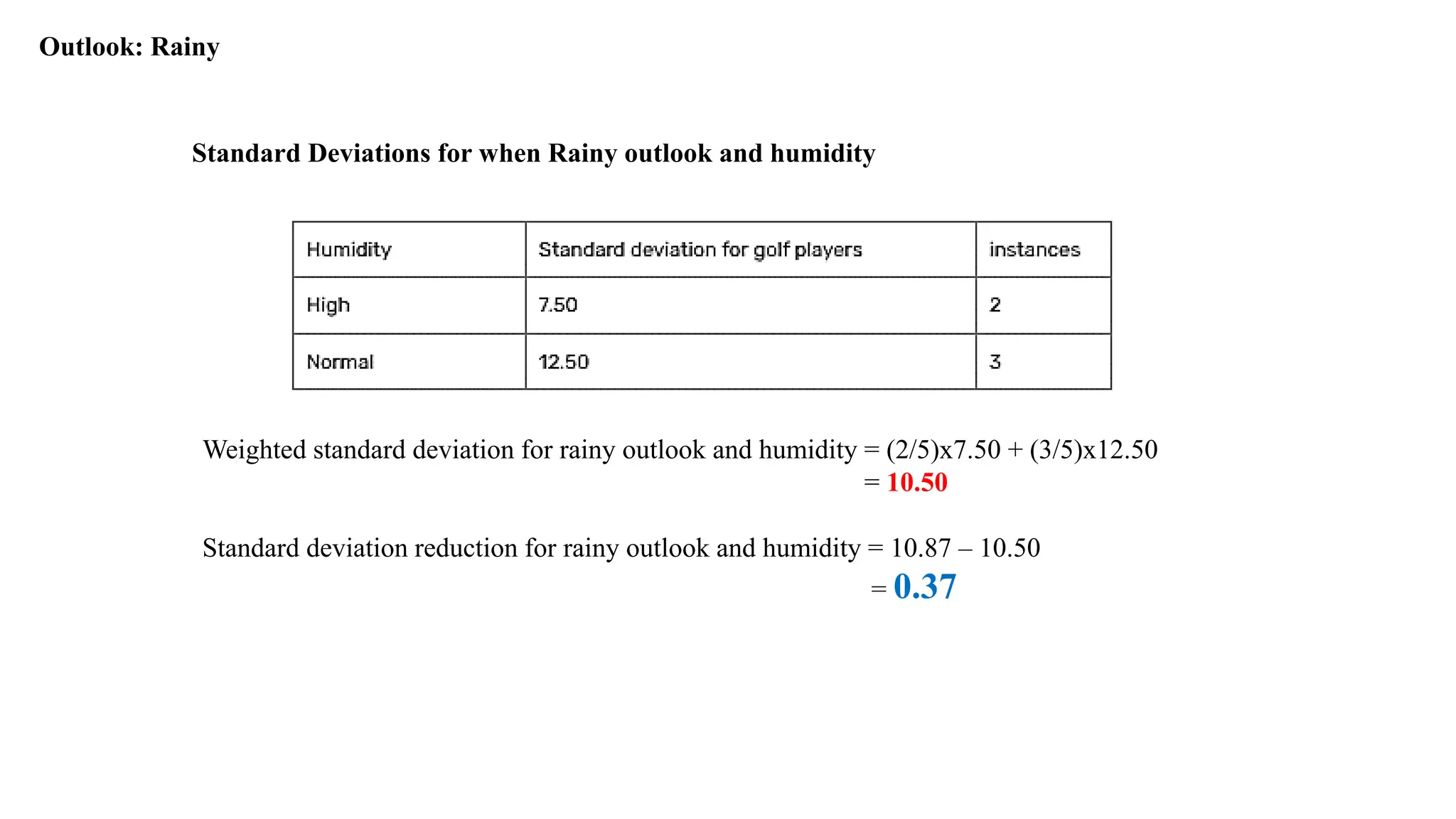
Outlook: Rainy
Standard Deviationsfor when Rainy outlook and humidity
Weighted standard deviation for rainy outlook and humidity = (2/5)x7.50 + (3/5)x12.50
= 10.50
Standard deviation reduction for rainy outlook and humidity = 10.87 – 10.50
= 0.37
101.
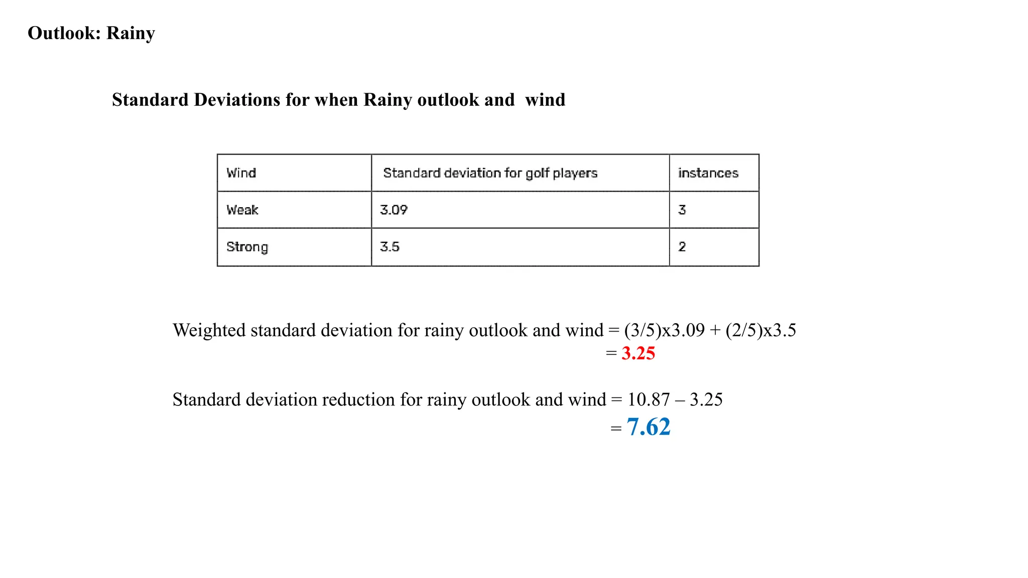
Outlook: Rainy
Standard Deviationsfor when Rainy outlook and wind
Weighted standard deviation for rainy outlook and wind = (3/5)x3.09 + (2/5)x3.5
= 3.25
Standard deviation reduction for rainy outlook and wind = 10.87 – 3.25
= 7.62

![Entropy in binary classification
Entropy measures the impurity of a collection of examples.
It depends from the distribution of the random variable p.
S is a collection of training examples
p+ the proportion of positive examples in S
p– the proportion of negative examples in S
Entropy (S) – p+ log2 p+ – p– log2 p– [0 log20 = 0]
Entropy ([14+, 0–]) = – 14/14 log2 (14/14) – 0 log2 (0) = 0
Entropy ([9+, 5–]) = – 9/14 log2 (9/14) – 5/14 log2 (5/14) = 0.94
Entropy ([7+, 7– ]) = – 7/14 log2 (7/14) – 7/14 log2 (7/14) = 1/2 + 1/2 = 1
Note: the log of a number < 1 is negative, 0 p 1, 0 entropy 1](https://image.slidesharecdn.com/module3-decisiontree-250524144550-934a5ab1/75/Decision-Tree-ID3-C4-5-CART-Regression-Tree-13-2048.jpg)
![Entropy in general
• Entropy measures the amount of information in a random variable
H(X) = – p+ log2 p+ – p– log2 p– X = {+, –}
for binary classification [two-valued random variable]
c c
H(X) = – pi log2 pi = pi log2 1/ pi X = {i, …, c}
i=1 i=1
for classification in c classes
Example: rolling a die with 8, equally probable, sides
8
H(X) = – 1/8 log2 1/8 = – log2 1/8 = log2 8 = 3
i=1](https://image.slidesharecdn.com/module3-decisiontree-250524144550-934a5ab1/75/Decision-Tree-ID3-C4-5-CART-Regression-Tree-14-2048.jpg)

![Example: Expected Information Gain
Let
Values(Wind) = {Weak, Strong}
S = [9+, 5−]
SWeak = [6+, 2−]
SStrong = [3+, 3−]
Information gain due to knowing Wind:
Gain(S, Wind) = Entropy(S) − 8/14 Entropy(SWeak) − 6/14 Entropy(SStrong)
= 0.94 − 8/14 0.811 − 6/14 1.00
= 0.048](https://image.slidesharecdn.com/module3-decisiontree-250524144550-934a5ab1/75/Decision-Tree-ID3-C4-5-CART-Regression-Tree-18-2048.jpg)
![Calculate Standard deviation
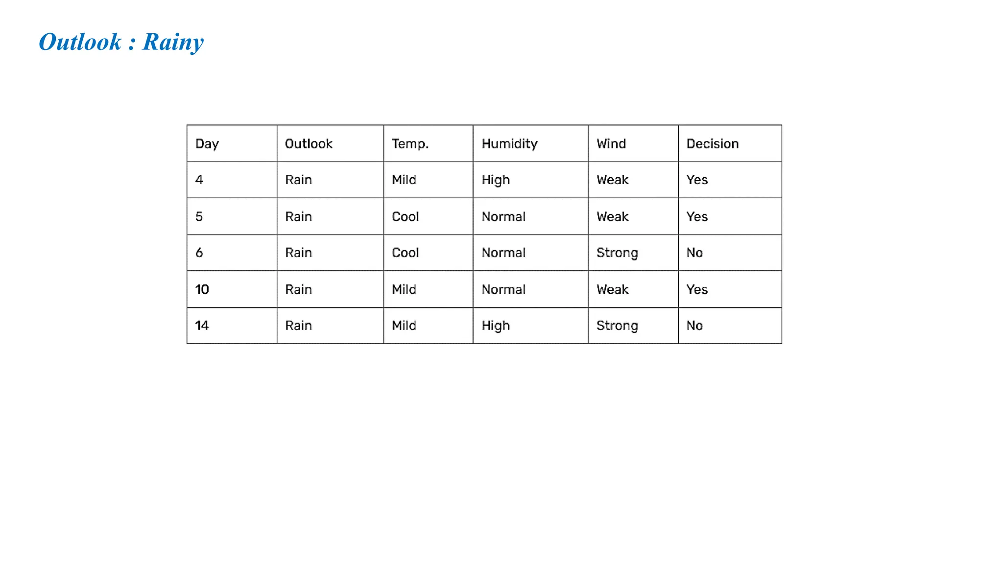
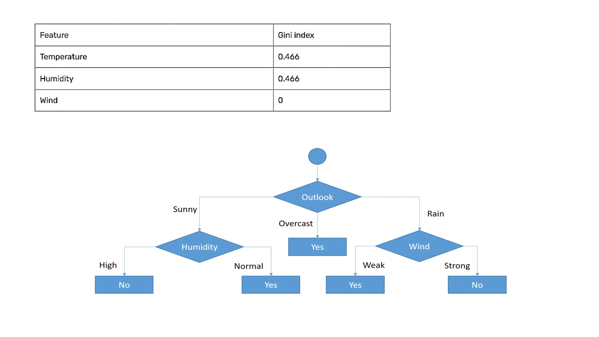
Golf players = {25, 30, 46, 45, 52, 23, 43, 35, 38, 46, 48, 52, 44, 30}
Average of golf players = (25 + 30 + 46 + 45 + 52 + 23 + 43 + 35 + 38 + 46 + 48 + 52 + 44 + 30 )/14 = 39.78
Standard deviation of golf players = √[( (25 – 39.78)2 + (30 – 39.78)2 + (46 – 39.78)2 + … + (30 – 39.78)2 )/14]
= 9.32](https://image.slidesharecdn.com/module3-decisiontree-250524144550-934a5ab1/75/Decision-Tree-ID3-C4-5-CART-Regression-Tree-76-2048.jpg)