Downloaded 107 times


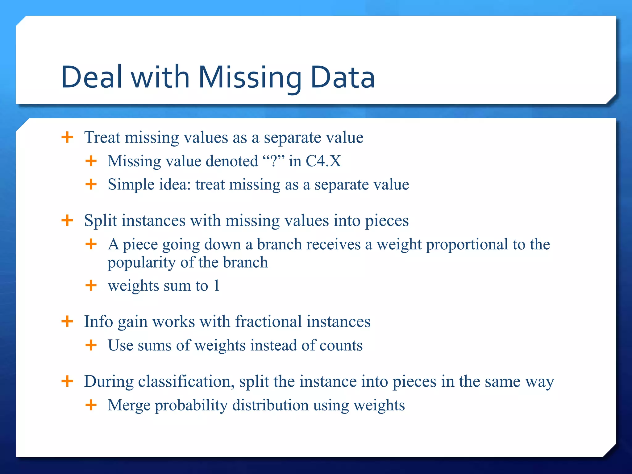
![Deal with continuous attributes
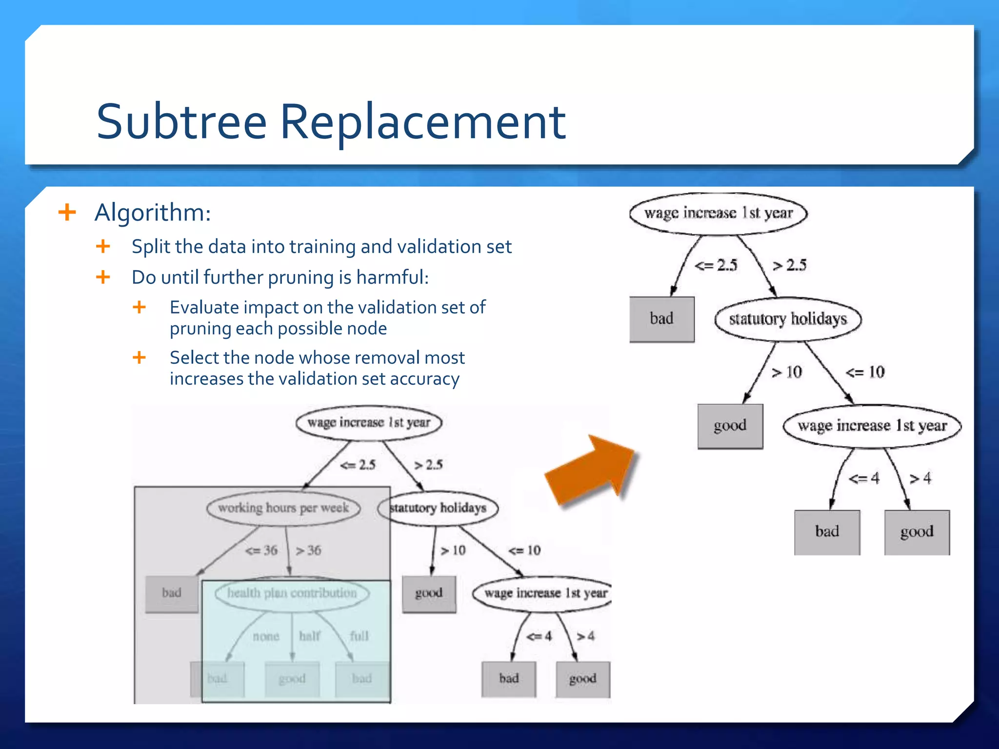
Split on temperature attribute:
E.g.: temperature < 71.5: yes/4, no/2
temperature ≥ 71.5: yes/5, no/3
Info([4,2],[5,3]) = 6/14 info([4,2]) + 8/14 info([5,3]) = 0.939 bits
Place split points halfway between values
Can evaluate all split points in one pass!](https://image.slidesharecdn.com/119d54be-5ab0-4ad8-b094-297da31793e2-160222065850/75/Decision-Tree-C4-5-CART-14-2048.jpg)
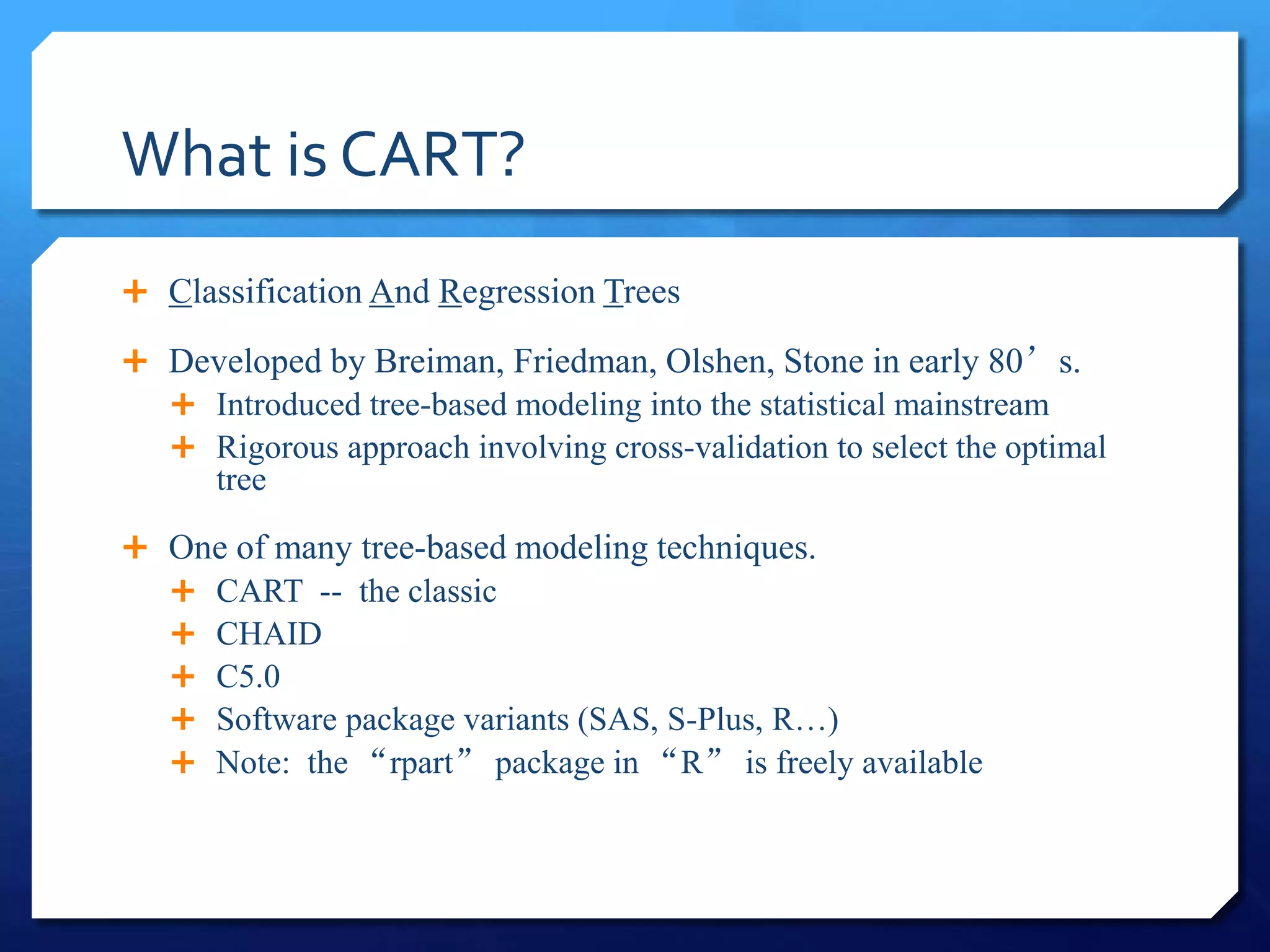
![RegressionTrees
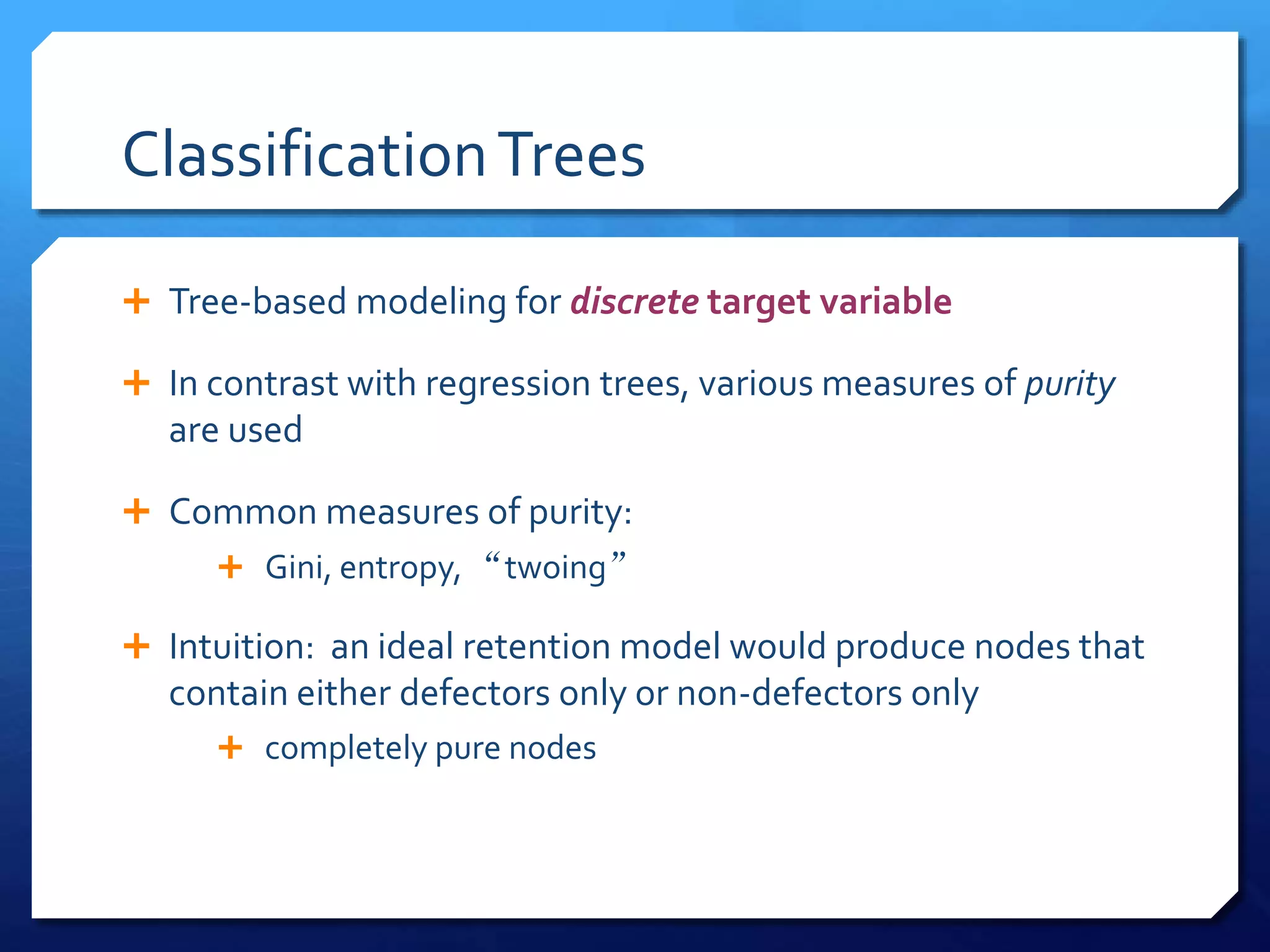
Tree-based modeling for continuous target variable
most intuitively appropriate method for loss ratio analysis
Find split that produces greatest separation in
∑[y – E(y)]2
i.e.: find nodes with minimal within variance
and therefore greatest between variance
like credibility theory
Every record in a node is assigned the same yhat
model is a step function](https://image.slidesharecdn.com/119d54be-5ab0-4ad8-b094-297da31793e2-160222065850/75/Decision-Tree-C4-5-CART-20-2048.jpg)
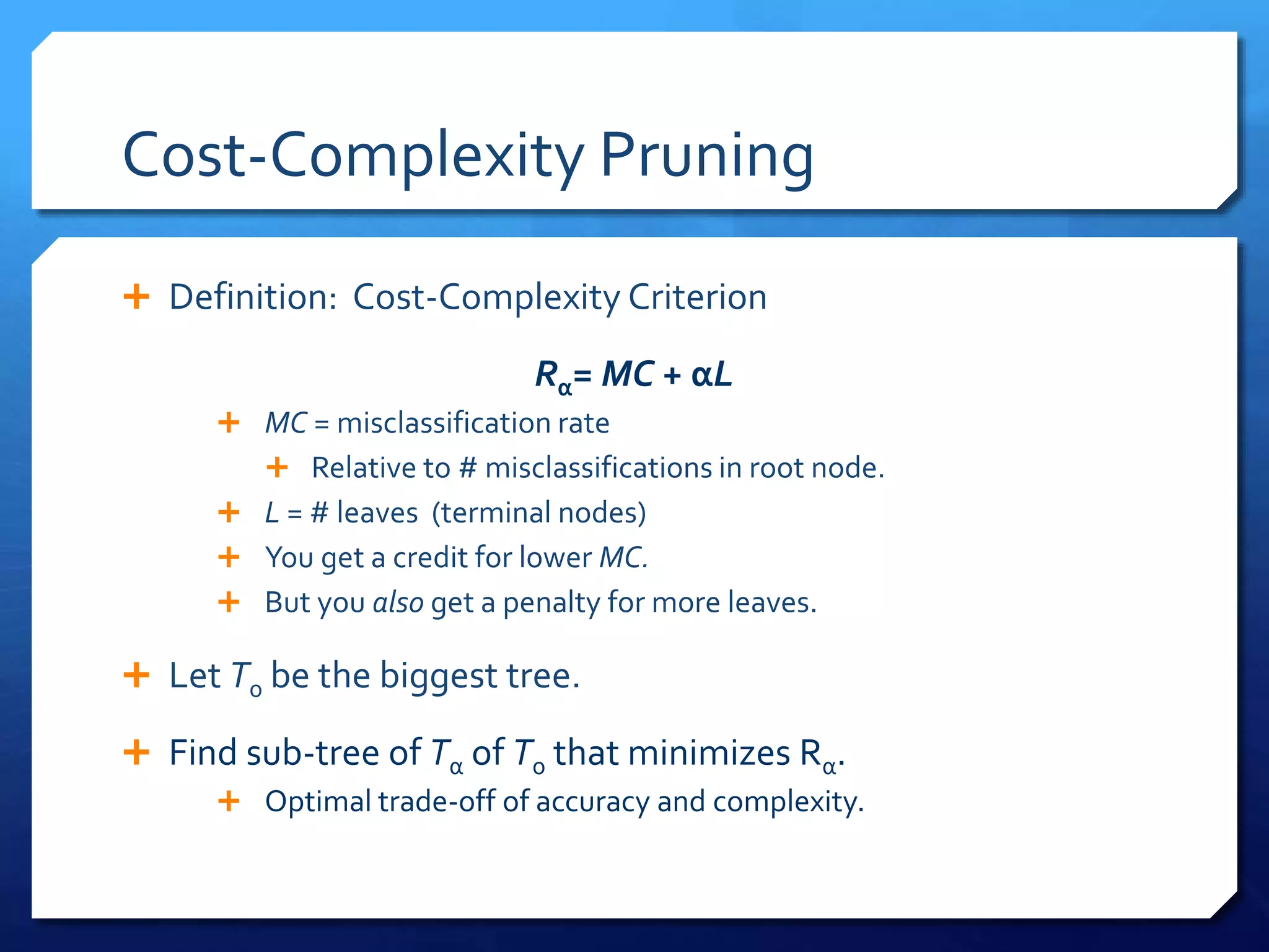


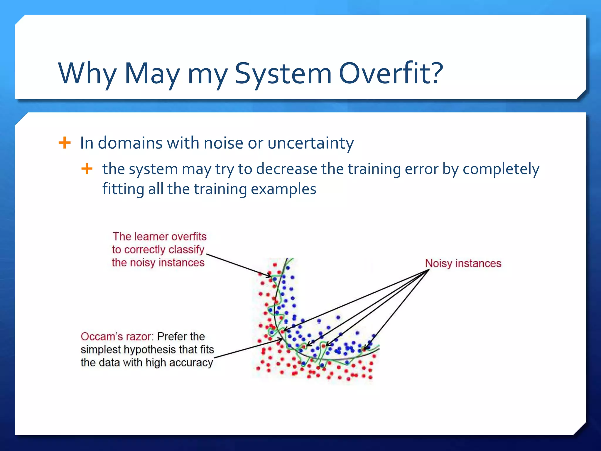
This document discusses decision tree algorithms C4.5 and CART. It explains that ID3 has limitations in dealing with continuous data and noisy data, which C4.5 aims to address through techniques like post-pruning trees to avoid overfitting. CART uses binary splits and measures like Gini index or entropy to produce classification trees, and sum of squared errors to produce regression trees. It also performs cost-complexity pruning to find an optimal trade-off between accuracy and model complexity.