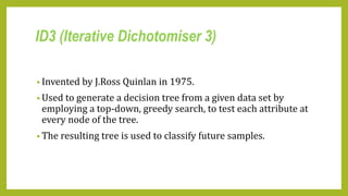
Decision trees are a type of supervised learning algorithm used for classification and regression. ID3 and C4.5 are algorithms that generate decision trees by choosing the attribute with the highest information gain at each step. Random forest is an ensemble method that creates multiple decision trees and aggregates their results, improving accuracy. It introduces randomness when building trees to decrease variance.

1. DECISION TREES

2. Contents
• Decision Trees
• ID3 Algorithm
• C 4.5 Algorithm
• Random Forest

3. Decision Trees
• Decision tree is a simple but powerful learning Paradigm.
• It is a type of classification algorithm for supervised learning.
• A decision tree is a tree in which each branch node represents
a choice between a number of alternatives and each leaf node
represents a decision.
• A node with outgoing edges is called an internal or test node.
All other nodes are called leaves (also known as terminal or
decision nodes).

4. Decision Trees

5. Construction of decision tree
1) First test all attributes and select the one that will function
as the best root.
2) Break-up the training set into subsets based on the
branches of the root node.
3) Test the remaining attributes to see which ones fit best
underneath the branches of the root node.
4) Continue this process for all other branches until

6. Decision Trees
I. All the examples of a subset are of one type.
II. There are no examples left.
III. There are no more attributes left.

7. Decision Tree Example
• Given a collection of shape and colour example, learn a
decision tree that represents it. Use this representation to
classify new examples.

8. 8
• Decision Trees are classifiers for instances represented as
features vectors. (color = ;shape = ;label = )
• Nodes are tests for feature values;
• There is one branch for each value of the feature
• Leaves specify the categories (labels)
• Can categorize instances into multiple disjoint categories – multi-class
Color
Shape
Blue red Green
Shape
square
triangle circle circlesquare
AB
CA
B
B
Evaluation of a
Decision Tree
(color = RED ;shape = triangle)
Learning a
Decision Tree
Decision Trees: The Representation

9. 9
They can represent any Boolean function
• Can be rewritten as rules in Disjunctive Normal Form (DNF)
• green  square positive
• blue  circle  positive
• blue  square  positive
• The disjunction of these rules is equivalent to the Decision Tree
Color
Shape
Blue red Green
Shape
square
triangle circle circlesquare
-+
++
-
+
Binary classified Decision Trees

10. Limitation of Decision Trees
• Learning a tree that classifies the training data perfectly may
not lead to the tree with the best generalization performance.
- There may be noise in the training data the tree is fitting
- The algorithm might be making decisions based on
very little data.
• A hypothesis h is said to overfit the training data if there is
another hypothesis, h’, such that ‘h’ has smaller error than h’
on the training data but h has larger error on the test data than h’.

11. Decision Trees

12. Evaluation Methods for Decision Trees
• Two basic approaches
- Pre-pruning: Stop growing the tree at some point during
construction when it is determined that there is not enough
data to make reliable choices.
- Post-pruning: Grow the full tree and then remove nodes
that seem not to have sufficient evidence.
• Methods for evaluating subtrees to prune:
- Cross-validation: Reserve hold-out set to evaluate utility.
- Statistical testing: Test if the observed regularity can be
dismissed as likely to be occur by chance.
- Minimum Description Length: Is the additional complexity of
the hypothesis smaller than remembering the exceptions ?

13. ID3 (Iterative Dichotomiser 3)
• Invented by J.Ross Quinlan in 1975.
• Used to generate a decision tree from a given data set by
employing a top-down, greedy search, to test each attribute at
every node of the tree.
• The resulting tree is used to classify future samples.

16. TrainingSet Attributes Classes
Gender Car
Ownership
Travel Cost Income
Level
Transportation
Male 0 Cheap Low Bus
Male 1 Cheap Medium Bus
Female 1 Cheap Medium Train
Female 0 Cheap Low Bus
Male 1 Cheap Medium Bus
Male 0 Standard Medium Train
Female 1 Standard Medium Train
Female 1 Expensive High Car
Male 2 Expensive Medium Car
Female 2 Expensive High Car

17. Algorithm
• Calculate the Entropy of every attribute using the data set.
• Split the set into subsets using the attribute for which entropy is
minimum (or, equivalently, information gain is maximum).
• Make a decision tree node containing that attribute.
• Recurse on subsets using remaining attributes.

18. Entropy
• In order to define Information Gain precisely, we need to discuss
Entropy first.
• A formula to calculate the homogeneity of a sample.
• A completely homogeneous sample has entropy of 0 (leaf node).
• An equally divided sample has entropy of 1.
• The formula for entropy is:
Entropy(S) = −𝑝(𝐼) log2 𝑝(𝐼)
• where p(I) is the proportion of S belonging to class I. ∑ is over
total outcomes.

19. Entropy
• Example 1
If S is a collection of 14 examples with 9 YES and 5 NO
examples then
Entropy(S) = - (9/14) Log2 (9/14) - (5/14) Log2 (5/14)
= 0.940

20. Information Gain
• The information gain is based on the decrease in entropy after a
dataset is split on an attribute.
• The formula for calculating information gain is:
Gain(S, A) = Entropy(S) - ((|Sv| / |S|) * Entropy(Sv))
Where, Sv = subset of S for which attribute A has value v
• |Sv| = number of elements in Sv
• |S| = number of elements in S

21. Procedure
• First the entropy of the total dataset is calculated.
• The dataset is then split on the different attributes.
• The entropy for each branch is calculated.
• Then it is added proportionally, to get total entropy for the split.
• The resulting entropy is subtracted from the entropy before the
split.
• The result is the Information Gain, or decrease in entropy.
• The attribute that yields the largest IG is chosen for the decision
node.

22. Our Problem :

23. TrainingSet Attributes Classes
Gender Car
Ownership
Travel Cost Income
Level
Transportation
Male 0 Cheap Low Bus
Male 1 Cheap Medium Bus
Female 1 Cheap Medium Train
Female 0 Cheap Low Bus
Male 1 Cheap Medium Bus
Male 0 Standard Medium Train
Female 1 Standard Medium Train
Female 1 Expensive High Car
Male 2 Expensive Medium Car
Female 2 Expensive High Car

24. Calculate the entropy of the total dataset
• First compute the Entropy of given training set.
Probability
Bus : 4/10 = 0.4
Train: 3/10 = 0.3
Car:3/10 = 0.3
E(S) = -P(I) log2 P(I)
E(S) = -(0.4) log2 (0.4) – (0.3)log2 (0.3) – (0.3)log2 (0.3) = 1.571

26. Split the dataset on ‘Gender’ attribute
Probability
Bus : 3/5 = 0.6
Train: 1/5 = 0.2
Car:1/5 = 0.2
Probability
Bus : 1/5 = 0.2
Train: 2/5 = 0.4
Car:2/5 = 0.4
Gain(S,A) = E(S) – I(S,A)
I(S,A) = 1.522 *(5/10) +
1.371*(5/10)
Gain(S,A) = 1.571 – 1.447
= 0.12
E(Sv) = -0.6 log2 (0.6) – 0.2 log2 (0.2)- 0.2 log2 (0.2)
= 1.522
E(Sv) = -0.2 log2 (0.2) – 0.4 log2 (0.4)- 0.4 log2 (0.4)
= 1.371

28. Split the dataset on ‘ownership’ attribute
Probability
Bus : 2/3= 0.6
Train: 1/3 = 0.3
Car:0/3 = 0
Entropy = 0.918
Probability
Bus : 2/5 = 0.4
Train: 2/5 = 0.4
Car:1/5 = 0.2
Entropy = 1.522
Probability
Bus : 0/2 = 0
Train: 0/2 = 0
Car:2/2 = 1
Entropy = 0
Gain(S,A) = E(S) – I(S,A)
I(S,A) = 0.918 *(3/10) +
1.522*(5/10) + 0*(2/10)
Gain(S,A) = 1.571 – 1.0364
= 0.534

29. • If we choose Travel Cost as splitting attribute,
-Entropy for Cheap = 0.722
Standard = 0
Expensive = 0
IG = 1.21
• If we choose Income Level as splitting attribute,
-Entropy for Low = 0
Medium = 1.459
High = 0
IG = 0.695

30. Attribute Information
Gain
Gender 0.125
Car
Ownership
0.534
Travel Cost 1.21
Income Level 0.695

31. Diagram : Decision Tree
?
Travel
Cost
XpensivStandrdCheap
Train Car

32. Iteration on Subset of Training Set
Probability
Bus : 4/5 = 0.8
Train: 1/5 = 0.2
Car:0/5 = 0
E(S) = -P(I) log2 P(I)
E(S) = -(0.8) log2 (0.8) – (0.2)log2 (0.2) = 0.722

33. • If we choose Gender as splitting attribute,
-Entropy for Male = 0
Female = 1
IG = 0.322
• If we choose Car Ownership as splitting attribute,
-Entropy for 0 = 0
1 = 0.918
IG = 0.171
• If we choose Income Level as splitting attribute,
-Entropy for Low = 0
Medium = 0.918
IG = 0.171

34. Attributes Information
Gain
Gender 0.322
Car
Ownership
0.171
Income Level 0.171

35. Diagram : Decision Tree
Travel
Cost
XpensivStandrdCheap
Train CarMale Female
Bus 0 1
Train Bus

36. Solution to Our Problem :
Name Gender Car
Ownership
Travel Cost Income
Level
Transportat
ion
Abhi Male 1 Standard High Train
Pavi Male 0 Cheap Medium Bus
Ammu Female 1 Cheap High Bus

37. Drawbacks of ID3
• Data may be over-fitted or over-classified, if a small sample is
tested.
• Only one attribute at a time is tested for making a decision.
• Classifying continuous data may be computationally
expensive.
• Does not handle numeric attributes and missing values.

38. C4.5 Algorithm
• This algorithm is also invented by J.Ross Quinlan., for generating
decision tree.
• It can be treated as an extension of ID3.
• C4.5 is mainly used for classification of data.
• It is called statistical classifier because of its potential for handling noisy
data.

39. Construction
• Base cases are determined.
• For each attribute a, the normalized information gain is found
out by splitting on a.
• Let a-best be the attribute with the highest normalized
information gain.
• Create a decision node that split on a-best
• Recur on the sub-lists obtained by splitting on a-best, and add
those nodes as children of node.

40. • The new Features include,
(i) accepts both continuous and discrete features.
(ii) handles incomplete data points.
(iii) solves over-fitting problem by bottom-up technique
usually known as "pruning”.
(iv) different weights can be applied the features that comprise
the training data.

41. Application based on features
• Continuous attribute categorisation.
discretisation – It partitions the continuous attribute values
into discrete set of intervals.
• Handling missing values.
Uses the theory of probability – probability is calculated from
the observed frequencies, takes the best probable value after
computing the frequencies.

42. Random Forest
• Random forest is an ensemble classifier which uses many
decision trees.
• It builds multiple decision trees and merges them together to
get a more accurate and stable prediction.
• It can be used for both classification and regression problems.

43. Algorithm
1) Create a bootstrapped dataset.
2) Create a decision tree using the bootstrapped dataset, but
only use a random subset of variables(or columns) at each
step.
3) Go back to step 1 and repeat.
Using a bootstrapped sample and considering only a subset of
variables at each step results in a wide variety of trees.

44. Explanation
• First, the process starts with the randomisation of the data sets
(done by bagging)
• Bagging – helps to reduce the variance, helps in effective
classification.
• RF contains many classification trees.
• Bagging – Bootstrapping the data plus using the aggregate to
make a decision.
• Out-of-Bag-Dataset – The dataset formed by using un chosen
tuples from the training set during the process of bootstrapping.

45. Gini Index
• Random Forest uses the gini index taken from the CART learning
system to construct decision trees. The gini index of node
impurity is the measure most commonly chosen for
classification-type problems. If a dataset T contains examples
from n classes.
• gini index, Gini(T) is defined as:
Gini(T) = 1 - ∑ 𝑗=1
𝑛
𝑃𝑗
2
where pj is the relative frequency of class j in T

46. • If a dataset T is split into two subsets T1 and T2 with sizes N1
and N2 respectively, the gini index of the split data contains
examples from n classes, the gini index (T) is defined as:
• Ginisplit(T) = N1/Ngini(T1) + N2/Ngini(T2)

47. Flow Chart of Algorithm

48. Advantages
• It produces a highly accurate classifier and learning is fast
• It runs efficiently on large data bases.
• It can handle thousands of input variables without variable
deletion.
• It computes proximities between pairs of cases that can be
used in clustering, locating outliers or (by scaling) give
interesting views of the data.
• It offers an experimental method for detecting variable
interactions.