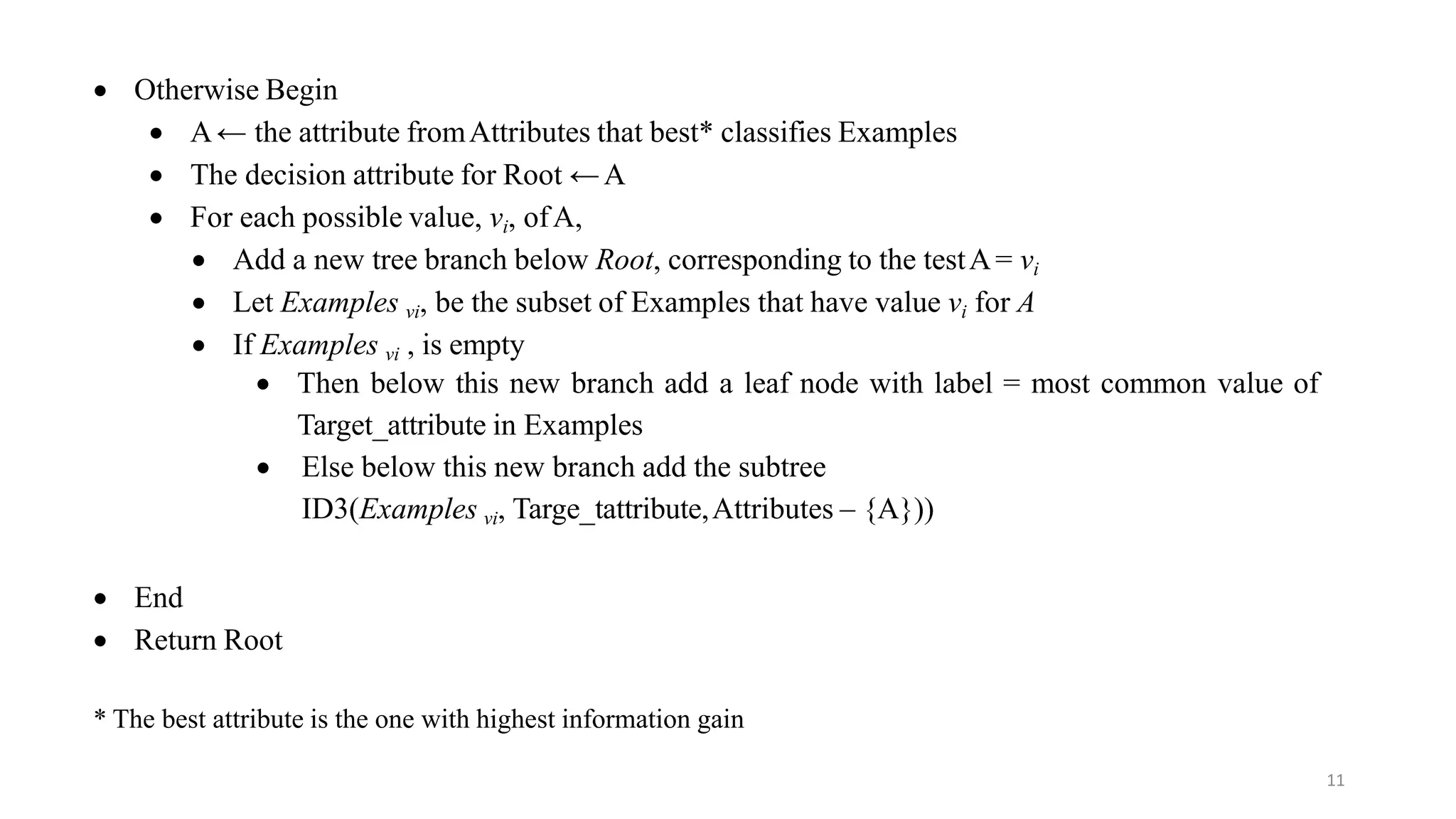
Decision tree learning involves creating a decision tree that classifies examples by sorting them from the root node to a leaf node. Each node tests an attribute and branches correspond to attribute values. Instances are classified by traversing the tree in this way. The ID3 algorithm uses information gain to select the attribute that best splits examples at each node, creating a greedy top-down search through possible trees. It calculates information gain, which measures the expected reduction in entropy (impurity), to determine which attribute best classifies examples at each step.

1. MODULE -3
DECISION TREE LEARNING
1

2. Decision tree learning is a method for approximating
discrete-valued target functions, in which the learned
function is represented by a decision tree.
2

3. DECISION TREE REPRESENTATION
FIGURE: A
decision tree for the
concept PlayTennis.
An example is
classified by sorting
it through the tree to
the appropriate leaf
node, then returning
the classification
associated with this
leaf
3

4. 4
• Decision trees classify instances by sorting them down the tree from the root to
some leaf node, which provides the classification of the instance.
• Each node in the tree specifies a test of some attribute of the instance, and each
branch descending from that node corresponds to one of the possible values for
this attribute.
• An instance is classified by starting at the root node of the tree, testing the
attribute specified by this node, then moving down the tree branch corresponding
to the value of the attribute in the given example. This process is then repeated
for the subtree rooted at the new node.

5. 5
• Decision trees represent a disjunction of conjunctions of constraints on the
attribute values of instances.
• Each path from the tree root to a leaf corresponds to a conjunction of attribute
tests, and the tree itself to a disjunction of these conjunctions
For example,
The decision tree shown in above figure corresponds to the expression
(Outlook = Sunny 𝖠 Humidity = Normal)
𝗏
𝗏
(Outlook = Overcast)
(Outlook = Rain 𝖠 Wind = Weak)

6. 6
APPROPRIATE PROBLEMS FOR
DECISION TREE LEARNING
Decision tree learning is generally best suited to problems with the following
characteristics:
1. Instances are represented by attribute-value pairs – Instances are described by
a fixed set of attributes and their values
2. The target function has discrete output values – The decision tree assigns a
Boolean classification (e.g., yes or no) to each example. Decision tree methods
easily extend to learning functions with more than two possible output values.
3. Disjunctive descriptions may be required

7. 7
4. The training data may contain errors – Decision tree learning methods are
robust to errors, both errors in classifications of the training examples and errors
in the attribute values that describe these examples.
5. The training data may contain missing attribute values – Decision tree
methods can be used even when some training examples have unknown values
• Decision tree learning has been applied to problems such as learning to classify
medical patients by their disease, equipment malfunctions by their cause, and
loan applicants by their likelihood of defaulting on payments.
• Such problems, in which the task is to classify examples into one of a discrete set
of possible categories, are often referred to as classification problems.

8. 8
THE BASIC DECISION TREE LEARNING
ALGORITHM
• Most algorithms that have been developed for learning decision trees are
variations on a core algorithm that employs a top-down, greedy search through the
space of possible decision trees. This approach is exemplified by the ID3
algorithm and its successor C4.5

9. 9
What is the ID3 algorithm?
• ID3 stands for Iterative Dichotomiser 3
• ID3 is a precursor to the C4.5Algorithm.
• The ID3 algorithm was invented by Ross Quinlan in 1975
• Used to generate a decision tree from a given data set by employing a top-down,
greedy search, to test each attribute at every node of the tree.
• The resulting tree is used to classify future samples.

10. 10
ID3 algorithm
ID3(Examples, Target_attribute,Attributes)
Examples are the training examples. Target_attribute is the attribute whose value is to be predicted
by the tree. Attributes is a list of other attributes that may be tested by the learned decision tree.
Returns a decision tree that correctly classifies the given Examples.
 Create a Root node for the tree
 If all Examples are positive, Return the single-node tree Root, with label = +
 If all Examples are negative, Return the single-node tree Root, with label = -
 If Attributes is empty, Return the single-node tree Root, with label = most common value of
Target_attribute in Examples

11. 11
 Otherwise Begin
 A← the attribute fromAttributes that best* classifies Examples
 The decision attribute for Root ←A
 For each possible value, vi, ofA,
 Add a new tree branch below Root, corresponding to the testA= vi
 Let Examples vi, be the subset of Examples that have value vi for A
 If Examples vi , is empty
 Then below this new branch add a leaf node with label = most common value of
Target_attribute in Examples
 Else below this new branch add the subtree
ID3(Examples vi, Targe_tattribute,Attributes – {A}))
 End
 Return Root
* The best attribute is the one with highest information gain

12. 12
Which Attribute Is the Best Classifier?
• The central choice in the ID3 algorithm is selecting which attribute to test at each
node in the tree.
• A statistical property called information gain that measures how well a given
attribute separates the training examples according to their target classification.
• ID3 uses information gain measure to select among the candidate attributes at
each step while growing the tree.

13. ENTROPY MEASURES HOMOGENEITY OF EXAMPLES
• To define information gain, we begin by defining a measure called entropy.
Entropy measures the impurity of a collection of examples.
• Given a collection S, containing positive and negative examples of some target
concept, the entropy of S relative to this Boolean classification is
Where,
p+ is the proportion of positive examples in S
p- is the proportion of negative examples in S.
13

14. Example: Entropy
• Suppose S is a collection of 14 examples of some boolean concept, including 9
positive and 5 negative examples. Then the entropy of S relative to this boolean
classification is
14

15. 15
• The entropy is 0 if all members of S belong to the same class
• The entropy is 1 when the collection contains an equal number of positive and
negative examples
• If the collection contains unequal numbers of positive and negative examples, the
entropy is between 0 and 1

16. 16

17. INFORMATION GAIN MEASURES THE EXPECTED
REDUCTION IN ENTROPY
• Information gain, is the expected reduction in entropy caused by partitioning the
examples according to this attribute.
• The information gain, Gain(S, A) of an attribute A, relative to a collection of
examples S, is defined as
17

18. 18
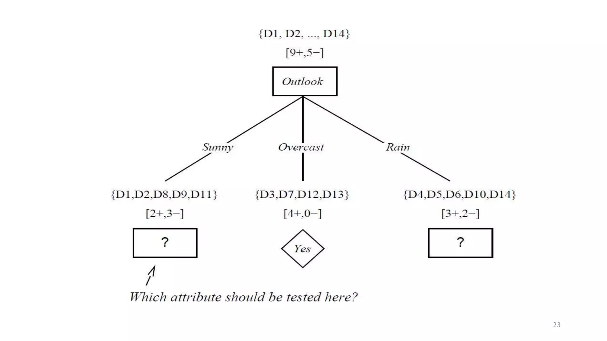
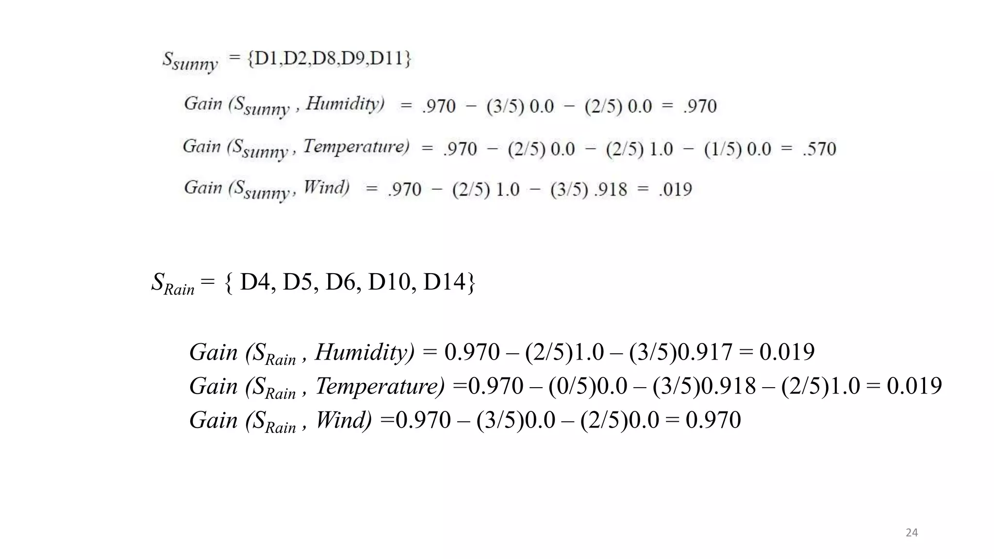
Example: Information gain
Let, Values(Wind) = {Weak, Strong}
S
SWeak
SStrong
= [9+, 5−]
= [6+, 2−]
= [3+, 3−]
Information gain of attribute Wind:
Gain(S, Wind) = Entropy(S) − 8/14 Entropy (SWeak) − 6/14 Entropy (SStrong)
= 0.94 – (8/14)* 0.811 – (6/14) *1.00
= 0.048

19. 19
An Illustrative Example
• To illustrate the operation of ID3, consider the learning task represented by the
training examples of below table.
• Here the target attribute PlayTennis, which can have values yes or no for
different days.
• Consider the first step through the algorithm, in which the topmost node of the
decision tree is created.

20. 20
Day Outlook Temperature Humidity Wind PlayTennis
D1 Sunny Hot High Weak No
D2 Sunny Hot High Strong No
D3 Overcast Hot High Weak Yes
D4 Rain Mild High Weak Yes
D5 Rain Cool Normal Weak Yes
D6 Rain Cool Normal Strong No
D7 Overcast Cool Normal Strong Yes
D8 Sunny Mild High Weak No
D9 Sunny Cool Normal Weak Yes
D10 Rain Mild Normal Weak Yes
D11 Sunny Mild Normal Strong Yes
D12 Overcast Mild High Strong Yes
D13 Overcast Hot Normal Weak Yes
D14 Rain Mild High Strong No

21. ID3 determines the information gain for each candidate attribute (i.e., Outlook,
Temperature, Humidity, and Wind), then selects the one with highest information
gain
21

22. 22
= 0.246
= 0.151
= 0.048
The information gain values for all four attributes are
• Gain(S, Outlook)
• Gain(S, Humidity)
• Gain(S, Wind)
• Gain(S, Temperature) = 0.029
• According to the information gain measure, the Outlook attribute provides the
best prediction of the target attribute, PlayTennis, over the training examples.
Therefore, Outlook is selected as the decision attribute for the root node, and
branches are created below the root for each of its possible values i.e., Sunny,
Overcast, and Rain.

23. 23

24. SRain = { D4, D5, D6, D10, D14}
Gain (SRain , Humidity) = 0.970 – (2/5)1.0 – (3/5)0.917 = 0.019
Gain (SRain , Temperature) =0.970 – (0/5)0.0 – (3/5)0.918 – (2/5)1.0 = 0.019
Gain (SRain , Wind) =0.970 – (3/5)0.0 – (2/5)0.0 = 0.970
24

25. 25