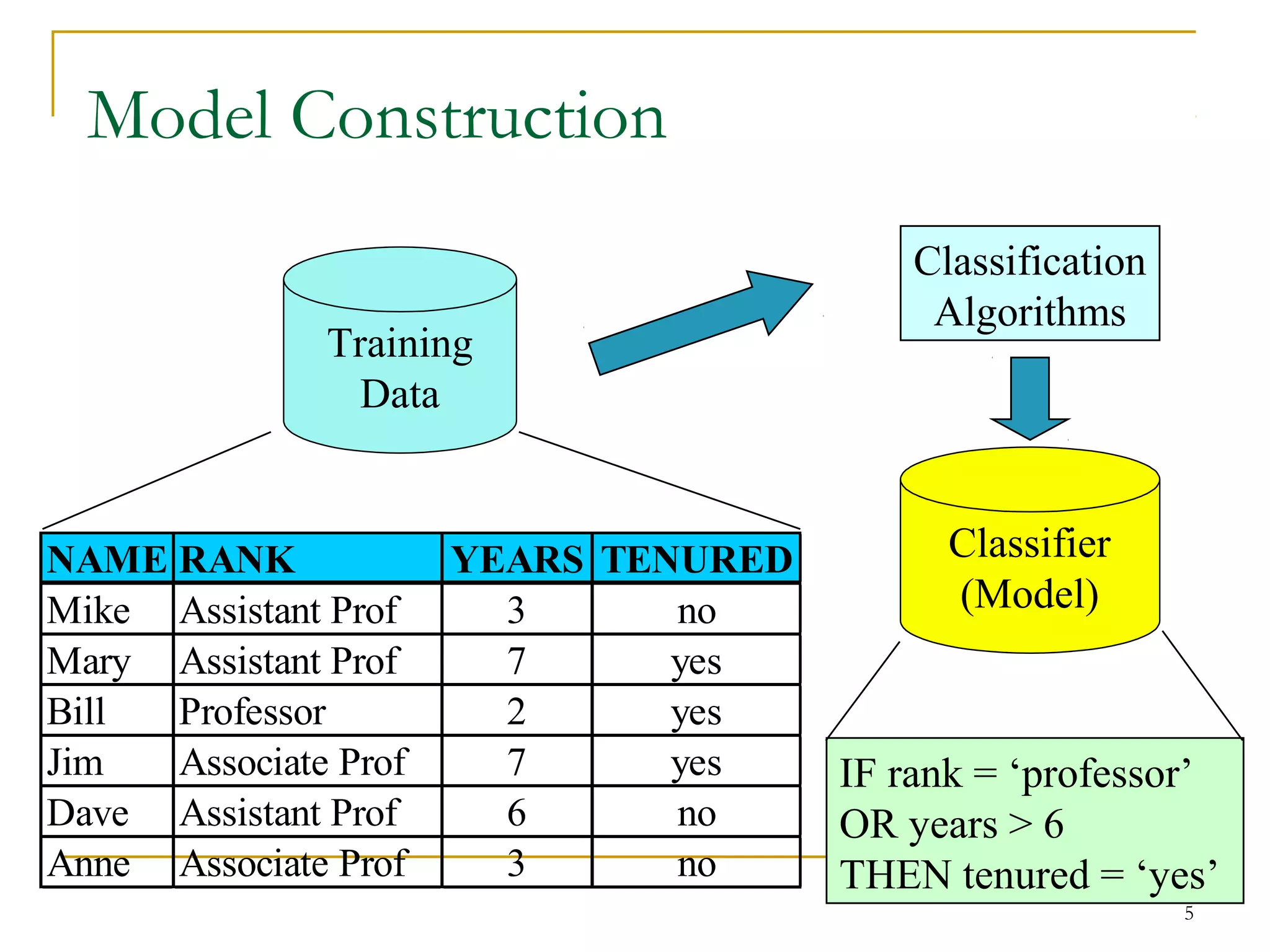
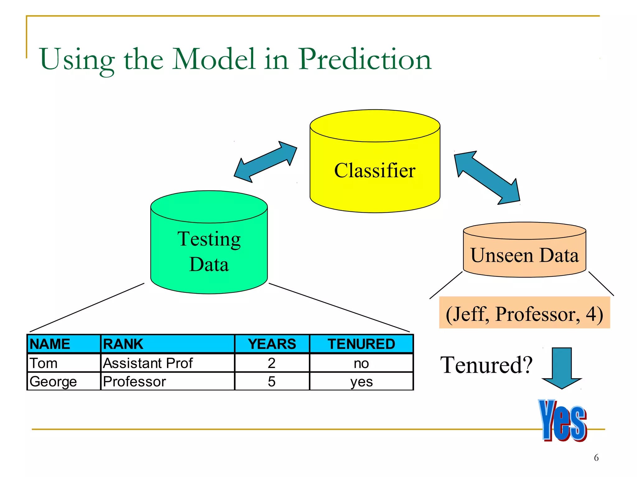
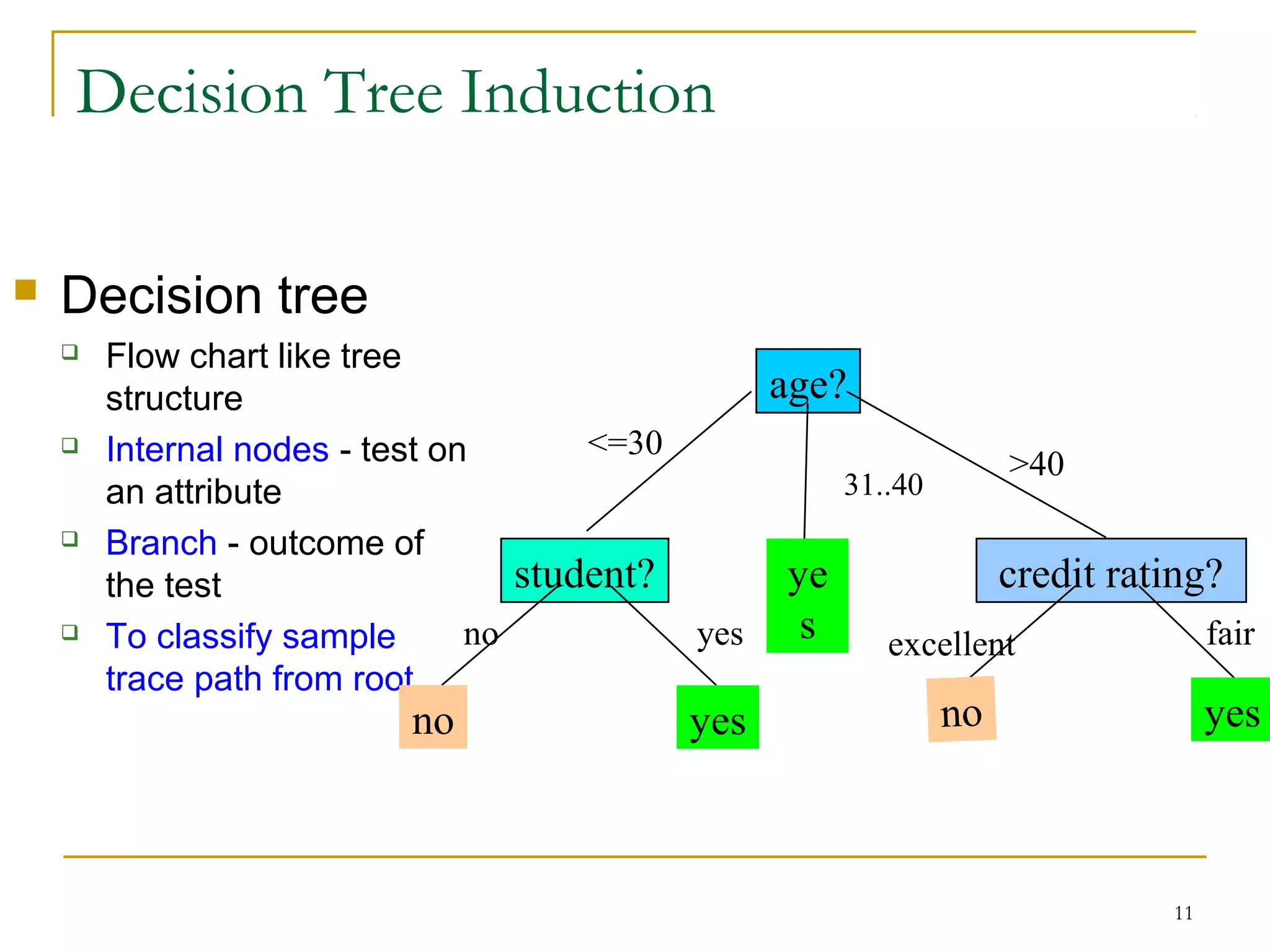
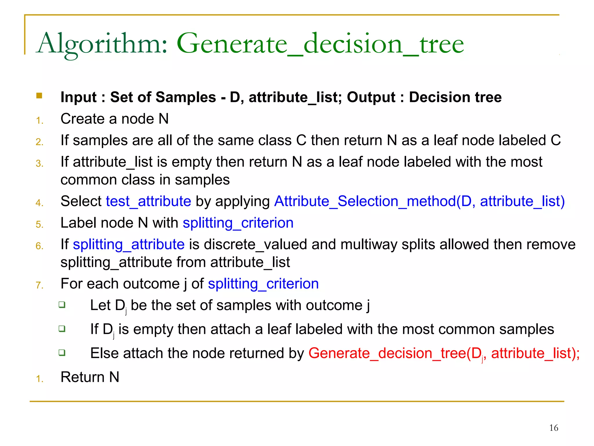
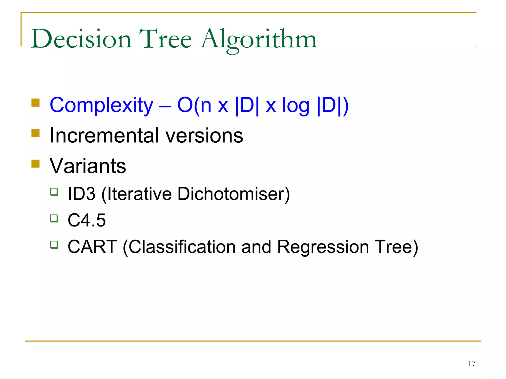
1
Classification
2
 Classification
 predicts categorical class labels (discrete or nominal)
 classifies data (constructs a model) based on the training set and the
values (class labels) in a classifying attribute and uses it in classifying
new data
 Prediction
 models continuous-valued functions, i.e., predicts unknown or missing
values
 Typical applications
 Credit approval
 Target marketing
 Medical diagnosis
 Fraud detection
Classification vs. Prediction
3
Classification—A Two-Step Process
 Model construction: describing a set of predetermined classes
 Each tuple/sample is assumed to belong to a predefined
class, as determined by the class label attribute
 The set of tuples used for model construction is training
set
 The model is represented as classification rules, decision
trees, or mathematical formulae
 Supervised Learning
4
Classification – A Two Step Process
 Model usage: for classifying future or unknown objects
 Estimate accuracy of the model
 The known label of test sample is compared with the
classified result from the model
 Accuracy rate is the percentage of test set samples that are
correctly classified by the model
 Test set is independent of training set, otherwise over-fitting
will occur
 If the accuracy is acceptable, use the model to classify data
tuples whose class labels are not known
5
Model Construction
Training
Data
NAME RANK YEARS TENURED
Mike Assistant Prof 3 no
Mary Assistant Prof 7 yes
Bill Professor 2 yes
Jim Associate Prof 7 yes
Dave Assistant Prof 6 no
Anne Associate Prof 3 no
Classification
Algorithms
IF rank = ‘professor’
OR years > 6
THEN tenured = ‘yes’
Classifier
(Model)
6
Using the Model in Prediction
Classifier
Testing
Data
NAME RANK YEARS TENURED
Tom Assistant Prof 2 no
George Professor 5 yes
Unseen Data
(Jeff, Professor, 4)
Tenured?
7
Supervised vs. Unsupervised Learning
 Supervised learning (classification)
 Supervision: The training data (observations, measurements,
etc.) are accompanied by labels indicating the class of the
observations
 New data is classified based on the training set
 Unsupervised learning (clustering)
 The class labels of training data is unknown
 Given a set of measurements, observations, etc. with the aim
of establishing the existence of classes or clusters in the data
8
Issues: Data Preparation
 Data cleaning
 Preprocess data in order to reduce noise and handle
missing values
 Relevance analysis (feature selection)
 Remove the irrelevant or redundant attributes
 Data transformation
 Generalize and/or normalize data
9
Issues: Evaluating Classification Methods
 Accuracy
 classifier accuracy: predicting class label
 predictor accuracy: guessing value of predicted attributes
 Speed
 time to construct the model (training time)
 time to use the model (classification/prediction time)
 Robustness
 handling noise and missing values
10
 Scalability
 efficiency in disk-resident databases
 Interpretability
 understanding and insight provided by the model
 Other measures, e.g., goodness of rules, such as
decision tree size or compactness of classification
rules
Issues: Evaluating Classification Methods
11
Decision Tree Induction
 Decision tree
 Flow chart like tree
structure
 Internal nodes - test on
an attribute
 Branch - outcome of
the test
 To classify sample
trace path from root
age?
student? credit rating?
<=30
>40
no yes yes
ye
s
31..40
no
fairexcellentyesno
12
Decision Tree Induction
 Basic algorithm (a greedy algorithm)
 Tree is constructed in a top-down recursive divide-and-conquer manner
 At start, all the training examples are at the root
 If all the samples belong to the same class the node becomes a leaf
labeled with the class else choose attribute for partitioning
 Attributes are categorical (if continuous-valued, they are discretized in
advance)
 Examples are partitioned recursively based on selected attributes
 Test attributes are selected on the basis of a heuristic or statistical
measure (e.g., information gain)
13
Attribute Selection
 Splitting Criteria
 determines the best way to split
 Indicates the splitting attribute and split point
 Measures
 Information Gain
 Gain Ratio
 Gini Index
14
Partitioning Scenarios
 Attribute:
 Discrete Valued
 A1, A2, A3.?
 Continuous Valued
 A <= Split point; A > Split point
 Discrete Valued and Binary tree must be produced
 A ∈ SA
15
Decision Tree Induction
 Conditions for stopping partitioning
 All samples for a given node belong to the same class
 There are no remaining attributes for further partitioning –
majority voting is employed for classifying the leaf
 There are no samples left
16
Algorithm: Generate_decision_tree
 Input : Set of Samples - D, attribute_list; Output : Decision tree
1. Create a node N
2. If samples are all of the same class C then return N as a leaf node labeled C
3. If attribute_list is empty then return N as a leaf node labeled with the most
common class in samples
4. Select test_attribute by applying Attribute_Selection_method(D, attribute_list)
5. Label node N with splitting_criterion
6. If splitting_attribute is discrete_valued and multiway splits allowed then remove
splitting_attribute from attribute_list
7. For each outcome j of splitting_criterion
 Let Dj be the set of samples with outcome j
 If Dj is empty then attach a leaf labeled with the most common samples
 Else attach the node returned by Generate_decision_tree(Dj, attribute_list);
1. Return N
17
Decision Tree Algorithm
 Complexity – O(n x |D| x log |D|)
 Incremental versions
 Variants
 ID3 (Iterative Dichotomiser)
 C4.5
 CART (Classification and Regression Tree)

2.1 Data Mining-classification Basic concepts

  • 1.
  • 2.
    2  Classification  predictscategorical class labels (discrete or nominal)  classifies data (constructs a model) based on the training set and the values (class labels) in a classifying attribute and uses it in classifying new data  Prediction  models continuous-valued functions, i.e., predicts unknown or missing values  Typical applications  Credit approval  Target marketing  Medical diagnosis  Fraud detection Classification vs. Prediction
  • 3.
    3 Classification—A Two-Step Process Model construction: describing a set of predetermined classes  Each tuple/sample is assumed to belong to a predefined class, as determined by the class label attribute  The set of tuples used for model construction is training set  The model is represented as classification rules, decision trees, or mathematical formulae  Supervised Learning
  • 4.
    4 Classification – ATwo Step Process  Model usage: for classifying future or unknown objects  Estimate accuracy of the model  The known label of test sample is compared with the classified result from the model  Accuracy rate is the percentage of test set samples that are correctly classified by the model  Test set is independent of training set, otherwise over-fitting will occur  If the accuracy is acceptable, use the model to classify data tuples whose class labels are not known
  • 5.
    5 Model Construction Training Data NAME RANKYEARS TENURED Mike Assistant Prof 3 no Mary Assistant Prof 7 yes Bill Professor 2 yes Jim Associate Prof 7 yes Dave Assistant Prof 6 no Anne Associate Prof 3 no Classification Algorithms IF rank = ‘professor’ OR years > 6 THEN tenured = ‘yes’ Classifier (Model)
  • 6.
    6 Using the Modelin Prediction Classifier Testing Data NAME RANK YEARS TENURED Tom Assistant Prof 2 no George Professor 5 yes Unseen Data (Jeff, Professor, 4) Tenured?
  • 7.
    7 Supervised vs. UnsupervisedLearning  Supervised learning (classification)  Supervision: The training data (observations, measurements, etc.) are accompanied by labels indicating the class of the observations  New data is classified based on the training set  Unsupervised learning (clustering)  The class labels of training data is unknown  Given a set of measurements, observations, etc. with the aim of establishing the existence of classes or clusters in the data
  • 8.
    8 Issues: Data Preparation Data cleaning  Preprocess data in order to reduce noise and handle missing values  Relevance analysis (feature selection)  Remove the irrelevant or redundant attributes  Data transformation  Generalize and/or normalize data
  • 9.
    9 Issues: Evaluating ClassificationMethods  Accuracy  classifier accuracy: predicting class label  predictor accuracy: guessing value of predicted attributes  Speed  time to construct the model (training time)  time to use the model (classification/prediction time)  Robustness  handling noise and missing values
  • 10.
    10  Scalability  efficiencyin disk-resident databases  Interpretability  understanding and insight provided by the model  Other measures, e.g., goodness of rules, such as decision tree size or compactness of classification rules Issues: Evaluating Classification Methods
  • 11.
    11 Decision Tree Induction Decision tree  Flow chart like tree structure  Internal nodes - test on an attribute  Branch - outcome of the test  To classify sample trace path from root age? student? credit rating? <=30 >40 no yes yes ye s 31..40 no fairexcellentyesno
  • 12.
    12 Decision Tree Induction Basic algorithm (a greedy algorithm)  Tree is constructed in a top-down recursive divide-and-conquer manner  At start, all the training examples are at the root  If all the samples belong to the same class the node becomes a leaf labeled with the class else choose attribute for partitioning  Attributes are categorical (if continuous-valued, they are discretized in advance)  Examples are partitioned recursively based on selected attributes  Test attributes are selected on the basis of a heuristic or statistical measure (e.g., information gain)
  • 13.
    13 Attribute Selection  SplittingCriteria  determines the best way to split  Indicates the splitting attribute and split point  Measures  Information Gain  Gain Ratio  Gini Index
  • 14.
    14 Partitioning Scenarios  Attribute: Discrete Valued  A1, A2, A3.?  Continuous Valued  A <= Split point; A > Split point  Discrete Valued and Binary tree must be produced  A ∈ SA
  • 15.
    15 Decision Tree Induction Conditions for stopping partitioning  All samples for a given node belong to the same class  There are no remaining attributes for further partitioning – majority voting is employed for classifying the leaf  There are no samples left
  • 16.
    16 Algorithm: Generate_decision_tree  Input: Set of Samples - D, attribute_list; Output : Decision tree 1. Create a node N 2. If samples are all of the same class C then return N as a leaf node labeled C 3. If attribute_list is empty then return N as a leaf node labeled with the most common class in samples 4. Select test_attribute by applying Attribute_Selection_method(D, attribute_list) 5. Label node N with splitting_criterion 6. If splitting_attribute is discrete_valued and multiway splits allowed then remove splitting_attribute from attribute_list 7. For each outcome j of splitting_criterion  Let Dj be the set of samples with outcome j  If Dj is empty then attach a leaf labeled with the most common samples  Else attach the node returned by Generate_decision_tree(Dj, attribute_list); 1. Return N
  • 17.
    17 Decision Tree Algorithm Complexity – O(n x |D| x log |D|)  Incremental versions  Variants  ID3 (Iterative Dichotomiser)  C4.5  CART (Classification and Regression Tree)