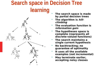
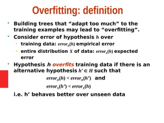
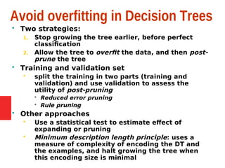
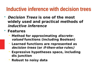
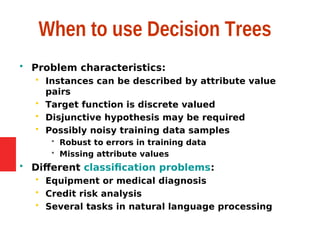
Decision tree learning is a method for approximating discrete-valued functions that is widely used in machine learning. It represents learned functions as decision trees that classify instances described by attribute value pairs. The ID3 algorithm performs a top-down induction of decision trees by selecting the attribute that best splits the data at each step. This results in an expressive hypothesis space that is robust to noise while avoiding overfitting through techniques like reduced-error pruning.

1. Decision Tree Learning
Dr. Radhey Shyam
Dept. Of CSE, BIET Lucknow
Email ID: shyam0058@gmail.com
Introduction To Machine Learning, Tom Mitchell,
Published by
Mc Graw-Hill International Editions, 199720/10/20

2. Inductive inference with decision trees
 Decision Trees is one of the most
widely used and practical methods of
inductive inference
 Features
 Method for approximating discrete-
valued functions (including Boolean)
 Learned functions are represented as
decision trees (or if-then-else rules)
 Expressive hypotheses space, including
dis junction
 Robust to noisy data

3. Decision tree representation
(Play Tennis)
Outlook=Sunny, Temp=Hot, Humidity=High, Wind=Strong No

4. Decision trees expressivity
 Decision trees represent a disjunction of
conjunctions on constraints on the value of
attributes:
(Outlook = Sunny  Humidity = Normal) 
(Outlook = Overcast) 
(Outlook = Rain  Wind = Weak)

5. Decision trees representation
+


6. When to use Decision Trees
 Problem characteristics:
 Instances can be described by attribute value
pairs
 Target function is discrete valued
 Disjunctive hypothesis may be required
 Possibly noisy training data samples
 Robust to errors in training data
 Missing attribute values
 Different classification problems:
 Equipment or medical diagnosis
 Credit risk analysis
 Several tasks in natural language processing

7. Top-down induction of DT
 ID3 (Quinlan, 1986) is a basic algorithm for
learning DT's
 Given a training set of examples, the algorithms
for building DT performs search in the space of
decision trees
 The construction of the tree is top-down. The
algorithm is greedy.
 The fundamental question is “which attribute
should be tested next? Which question gives us
more information?”
 Select the best attribute
 A descendent node is then created for each
possible value of this attribute and examples
are partitioned according to this value
 The process is repeated for each successor node
until all the examples are classified correctly or
there are no attributes left

8. Which attribute is the best
classifier?
 A statistical property called information gain,
measures how well a given attribute separates
the training examples
 Information gain uses the notion of entropy,
commonly used in information theory
 Information gain = expected reduction of
entropy

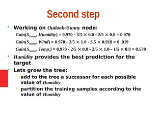
9. Entropy in binary classification
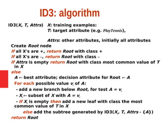
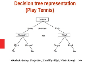
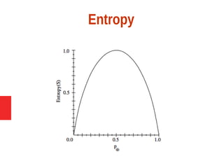
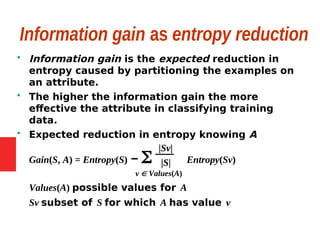
 Entropy measures the impurity of a collection of
examples. It depends from the distribution of the
random variable p.
 S is a collection of training examples
 p+ the proportion of positive examples in S
 p– the proportion of negative examples in S
Entropy (S)  – p+ log2 p+ – p–log2 p– [0 log20 = 0]
Entropy ([14+, 0–]) = –14/14 log2 (14/14) – 0log2 (0) = 0
Entropy ([9+, 5–]) = – 9/14 log2 (9/14) – 5/14 log2 (5/14) = 0.94
Entropy ([7+, 7– ]) = – 7/14 log2 (7/14) – 7/14log2 (7/14) =
= 1/2 + 1/2 = 1 [log21/2 = – 1]
Note: the log of a number < 1 is negative, 0  p  1, 0 
entropy  1

10. Entropy

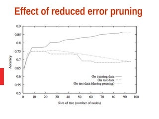
11. Entropy in general
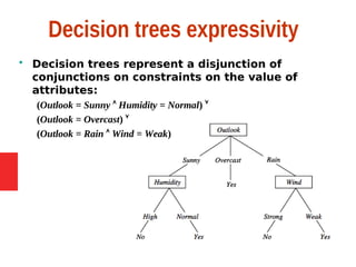
 Entropy measures the amount of information in
a random variable
H(X) = – p+ log2 p+ – p– log2 p– X = {+, –}
for binary classification [two-valued random
variable]
c c
H(X) = –  pi log2 pi =  pi log2 1/ pi X = {i, …, c}
i=1 i=1
for classification in c classes
Example: rolling a die with 8, equally probable,
sides
8
H(X) = –  1/8 log2 1/8 = – log2 1/8 = log2 8 = 3
i=1

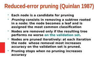
12. Entropy and information theory
 Entropy specifies the number the average length
(in bits) of the message needed to transmit the
outcome of a random variable. This depends on
the probability distribution.
 Optimal length code assigns  log2 p bits to
messages with probability p. Most probable
messages get shorter codes.
 Example: 8-sided [unbalanced] die
1 2 3 4 5 6 7 8
4/16 4/16 2/16 2/16 1/16 1/16 1/16 1/16
2 bits 2 bits 3 bits 3 bits 4bits 4bits 4bits 4bits
E = (1/4 log2 4)  2 + (1/8 log2 8)  2 + (1/16 log2 16)  4 = 1+3/4+1 =
2.75

13. Information gain as entropy reduction
 Information gain is the expected reduction in
entropy caused by partitioning the examples on
an attribute.
 The higher the information gain the more
effective the attribute in classifying training
data.
 Expected reduction in entropy knowing A
Gain(S, A) = Entropy(S) −  Entropy(Sv)
v  Values(A)
Values(A) possible values for A
Sv subset of S for which A has value v
|Sv|
|S|

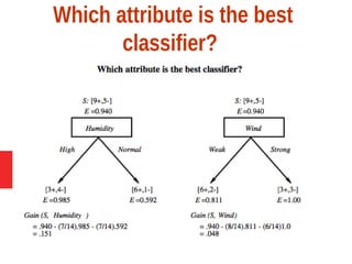
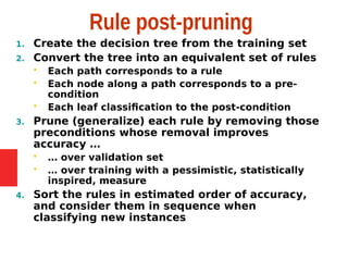
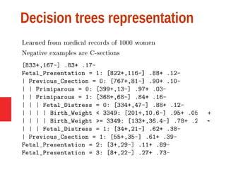
14. Example: expected information
gain
 Let
 Values(Wind) = {Weak, Strong}
 S = [9+, 5−]
 SWeak = [6+, 2−]
 SStrong = [3+, 3−]
 Information gain due to knowing Wind:
Gain(S, Wind) = Entropy(S) − 8/14 Entropy(SWeak) − 6/14 Entropy(SStrong)
= 0.94 − 8/14  0.811 − 6/14  1.00
= 0.048

15. Which attribute is the best
classifier?

16. Example

17. First step: which attribute to test at the
root?
 Which attribute should be tested at the root?
 Gain(S, Outlook) = 0.246
 Gain(S, Humidity) = 0.151
 Gain(S, Wind) = 0.084
 Gain(S, Temperature) = 0.029
 Outlook provides the best prediction for the
target
 Lets grow the tree:
 add to the tree a successor for each possible
value of Outlook
 partition the training samples according to the
value of Outlook

18. After first step

19. Second step
 Working on Outlook=Sunny node:
Gain(SSunny, Humidity) = 0.970  3/5  0.0  2/5  0.0 = 0.970
Gain(SSunny, Wind) = 0.970  2/5  1.0  3.5  0.918 = 0 .019
Gain(SSunny, Temp.) = 0.970  2/5  0.0  2/5  1.0  1/5  0.0 = 0.570
 Humidity provides the best prediction for the
target
 Lets grow the tree:
 add to the tree a successor for each possible
value of Humidity
 partition the training samples according to the
value of Humidity

20. Second and third steps
{D1, D2, D8}
No
{D9, D11}
Yes
{D4, D5, D10}
Yes
{D6, D14}
No

21. ID3: algorithm
ID3(X, T, Attrs) X: training examples:
T: target attribute (e.g. PlayTennis),
Attrs: other attributes, initially all attributes
Create Root node
If all X's are +, return Root with class +
If all X's are –, return Root with class –
If Attrs is empty return Root with class most common value of T
in X
else
A  best attribute; decision attribute for Root  A
For each possible value vi of A:
- add a new branch below Root, for test A = vi
- Xi  subset of X with A = vi
- If Xi is empty then add a new leaf with class the most
common value of T in X
else add the subtree generated by ID3(Xi, T, Attrs  {A})
return Root

22. Search space in Decision Tree
learning  The search space is made
by partial decision trees
 The algorithm is hill-
climbing
 The evaluation function is
information gain
 The hypotheses space is
complete (represents all
discrete-valued functions)
 The search maintains a
single current hypothesis
 No backtracking; no
guarantee of optimality
 It uses all the available
examples (not incremental)
 May terminate earlier,
accepting noisy classes

23. Inductive bias in decision tree
learning
 What is the inductive bias of DT learning?
1. Shorter trees are preferred over longer trees
Not enough. This is the bias exhibited by a
simple breadth first algorithm generating all
DT's e selecting the shorter one
2. Prefer trees that place high information gain
attributes close to the root
 Note: DT's are not limited in representing all
possible functions

24. Two kinds of biases
 Preference or search biases (due to the search
strategy)
 ID3 searches a complete hypotheses space; the
search strategy is incomplete
 Restriction or language biases (due to the set
of hypotheses expressible or considered)
 Candidate-Elimination searches an incomplete
hypotheses space; the search strategy is
complete
 A combination of biases in learning a linear
combination of weighted features in board
games.

25. Prefer shorter hypotheses: Occam's rasor
 Why prefer shorter hypotheses?
 Arguments in favor:
 There are fewer short hypotheses than long ones
 If a short hypothesis fits data unlikely to be a
coincidence
 Elegance and aesthetics
 Arguments against:
 Not every short hypothesis is a reasonable one.
 Occam's razor:"The simplest explanation is
usually the best one."
 a principle usually (though incorrectly)
attributed14th-century English logician and
Franciscan friar, William of Ockham.
 lex parsimoniae ("law of parsimony", "law of
economy", or "law of succinctness")
 The term razor refers to the act of shaving away
unnecessary assumptions to get to the simplest
explanation.

26. Issues in decision trees learning
 Over-fitting
 Reduced error pruning
 Rule post-pruning
 Extensions
 Continuous valued attributes
 Alternative measures for selecting attributes
 Handling training examples with missing attribute
values
 Handling attributes with different costs
 Improving computational efficiency
 Most of these improvements in C4.5 (Quinlan,
1993)

27. Overfitting: definition
 Building trees that “adapt too much” to the
training examples may lead to “overfitting”.
 Consider error of hypothesis h over
 training data: errorD(h) empirical error
 entire distribution X of data: errorX(h) expected
error
 Hypothesis h overfits training data if there is an
alternative hypothesis h'  H such that
errorD(h) < errorD(h’) and
errorX(h’) < errorX(h)
i.e. h’ behaves better over unseen data

28. Example
D15 Sunny Hot Normal Strong No

29. Overfitting in decision trees
Outlook=Sunny, Temp=Hot, Humidity=Normal, Wind=Strong, PlayTennis=No 
New noisy example causes splitting of second leaf node.

30. Overfitting in decision tree learning

31. Avoid overfitting in Decision Trees
 Two strategies:
1. Stop growing the tree earlier, before perfect
classification
2. Allow the tree to overfit the data, and then post-
prune the tree
 Training and validation set
 split the training in two parts (training and
validation) and use validation to assess the
utility of post-pruning
 Reduced error pruning
 Rule pruning
 Other approaches
 Use a statistical test to estimate effect of
expanding or pruning
 Minimum description length principle: uses a
measure of complexity of encoding the DT and
the examples, and halt growing the tree when
this encoding size is minimal

32. Reduced-error pruning (Quinlan 1987)
 Each node is a candidate for pruning
 Pruning consists in removing a subtree rooted
in a node: the node becomes a leaf and is
assigned the most common classification
 Nodes are removed only if the resulting tree
performs no worse on the validation set.
 Nodes are pruned iteratively: at each iteration
the node whose removal most increases
accuracy on the validation set is pruned.
 Pruning stops when no pruning increases
accuracy

33. Effect of reduced error pruning

34. Rule post-pruning
1. Create the decision tree from the training set
2. Convert the tree into an equivalent set of rules
 Each path corresponds to a rule
 Each node along a path corresponds to a pre-
condition
 Each leaf classification to the post-condition
3. Prune (generalize) each rule by removing those
preconditions whose removal improves
accuracy …
 … over validation set
 … over training with a pessimistic, statistically
inspired, measure
4. Sort the rules in estimated order of accuracy,
and consider them in sequence when
classifying new instances

35. Converting to rules
(Outlook=Sunny)(Humidity=High) (⇒ PlayTennis=No)

36. Why converting to rules?
 Each distinct path produces a different rule: a
condition removal may be based on a local
(contextual) criterion. Node pruning is global
and affects all the rules
 In rule form, tests are not ordered and there is
no book-keeping involved when conditions
(nodes) are removed
 Converting to rules improves readability for
humans

37. Dealing with continuous-valued
attributes
 So far discrete values for attributes and for outcome.
 Given a continuous-valued attribute A, dynamically
create a new attribute Ac
Ac = True if A < c, False otherwise
 How to determine threshold value c ?
 Example. Temperature in the PlayTennis example
 Sort the examples according to Temperature
Temperature 40 48 | 60 72 80 | 90
PlayTennis No No 54 Yes Yes Yes 85 No
 Determine candidate thresholds by averaging consecutive
values where there is a change in classification:
(48+60)/2=54 and (80+90)/2=85
 Evaluate candidate thresholds (attributes) according to
information gain. The best is Temperature>54.The new
attribute competes with the other ones.

38. Problems with information gain
 Natural bias of information gain: it favours
attributes with many possible values.
 Consider the attribute Date in the PlayTennis
example.
 Date would have the highest information gain since
it perfectly separates the training data.
 It would be selected at the root resulting in a very
broad tree
 Very good on the training, this tree would
perform poorly in predicting unknown instances.
Overfitting.
 The problem is that the partition is too specific,
too many small classes are generated.
 We need to look at alternative measures …

39. Handling incomplete training data
 How to cope with the problem that the value of
some attribute may be missing?
 Example: Blood-Test-Result in a medical
diagnosis problem
 The strategy: use other examples to guess
attribute
1. Assign the value that is most common among the
training examples at the node
2. Assign a probability to each value, based on
frequencies, and assign values to missing
attribute, according to this probability
distribution
 Missing values in new instances to be classified
are treated accordingly, and the most probable
classification is chosen (C4.5)

40. References
 Introduction to Machine Learning, Tom Mitchell,
Mc Graw-Hill International Editions, 1997.