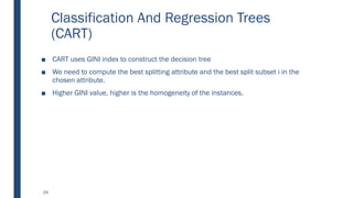
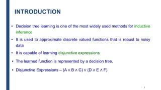
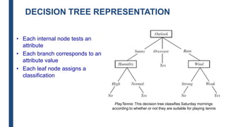
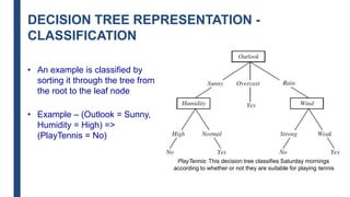
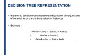
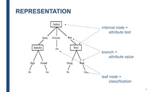
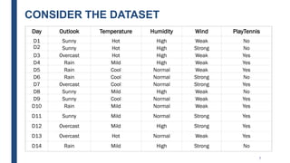
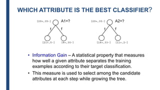
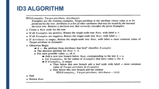
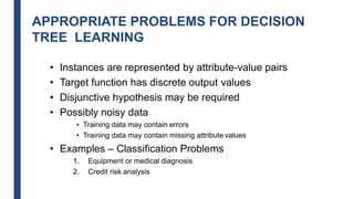
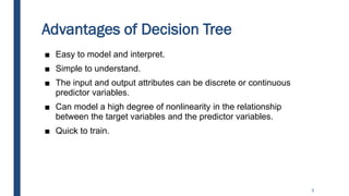
The document discusses decision tree learning, including: - Decision trees represent a disjunction of conjunctions of constraints on attribute values to classify instances. - The ID3 and C4.5 algorithms use information gain to select the attribute that best splits the data at each node, growing the tree in a top-down greedy manner. - Decision trees can model nonlinearity and are generally easy to interpret, but may overfit more complex datasets.

1. DECISION TREE
LEARNING
MODULE - 4
1

2. INTRODUCTION
• Decision tree learning is one of the most widely used methods for inductive
inference
• It is used to approximate discrete valued functions that is robust to noisy
data
• It is capable of learning disjunctive expressions
• The learned function is represented by a decision tree.
• Disjunctive Expressions – (A ∧ B ∧ C) ∨ (D ∧ E ∧ F)
2

3. REPRESENTATION
3
internal node =
attribute test
branch =
attribute value
leaf node =
classification

4. APPROPRIATE PROBLEMS FOR DECISION
TREE LEARNING
• Instances are represented by attribute-value pairs
• Target function has discrete output values
• Disjunctive hypothesis may be required
• Possibly noisy data
• Training data may contain errors
• Training data may contain missing attribute values
• Examples – Classification Problems
1. Equipment or medical diagnosis
2. Credit risk analysis

5. Advantages of Decision Tree
■ Easy to model and interpret.
■ Simple to understand.
■ The input and output attributes can be discrete or continuous
predictor variables.
■ Can model a high degree of nonlinearity in the relationship
between the target variables and the predictor variables.
■ Quick to train.
5

6. Disadvantages of Decision Tree
■ Issues arising with decision tree learning
– Difficult to determine when to stop growing the tree
– If training data has errors or missing values, decision tree
becomes biased or unstable.
– If training data is continuous valued attributes, handling it is
computationally complex and has to be discretized.
– A complex decision tree may be over fitting.
6

7. CONSIDER THE DATASET
7
Day Outlook Temperature Humidity Wind PlayTennis
D1 Sunny Hot High Weak No
D2 Sunny Hot High Strong No
D3 Overcast Hot High Weak Yes
D4 Rain Mild High Weak Yes
D5 Rain Cool Normal Weak Yes
D6 Rain Cool Normal Strong No
D7 Overcast Cool Normal Strong Yes
D8 Sunny Mild High Weak No
D9 Sunny Cool Normal Weak Yes
D10 Rain Mild Normal Weak Yes
D11 Sunny Mild Normal Strong Yes
D12 Overcast Mild High Strong Yes
D13 Overcast Hot Normal Weak Yes
D14 Rain Mild High Strong No

8. DECISION TREE REPRESENTATION
• Each internal node tests an
attribute
• Each branch corresponds to an
attribute value
• Each leaf node assigns a
classification
PlayTennis: This decision tree classifies Saturday mornings
according to whether or not they are suitable for playing tennis

9. DECISION TREE REPRESENTATION -
CLASSIFICATION
• An example is classified by
sorting it through the tree from
the root to the leaf node
• Example – (Outlook = Sunny,
Humidity = High) =>
(PlayTennis = No)
PlayTennis: This decision tree classifies Saturday mornings
according to whether or not they are suitable for playing tennis

10. DECISION TREE REPRESENTATION
• In general, decision trees represent a disjunction of conjunctions
of constraints on the attribute values of instances
• Example –

11. TOP-DOWN INDUCTION OF DECISION TREES
1. Find A = the best decision attribute for next node
2. Assign A as decision attribute for node
3. For each value of A create new descendants of node
4. Sort the training examples to the leaf node.
5. If training examples classified perfectly, STOP else
iterate over the new leaf nodes.

12. WHICH ATTRIBUTE IS THE BEST CLASSIFIER?
• Information Gain – A statistical property that measures
how well a given attribute separates the training
examples according to their target classification.
• This measure is used to select among the candidate
attributes at each step while growing the tree.

13. DECISION TREE ALGORITHMS
• Decision tree algorithms employs top-down greedy
search through the space of possible decision trees
• ID3 (Iterative Dichotomizer 3) by Quinlan 1986, and
C4.5 by Quinlan 1986 uses this approach
• Most algorithms that have been developed for
learning decision trees are variations of the core
algorithms

14. BASIC ID3 LEARNING ALGORITHM APPROACH
• Top-down construction of the tree, beginning with the question "which
attribute should be tested at the root of the tree?'
• Each instance attribute is evaluated using a statistical test to determine
how well it alone classifies the training examples.
• The best attribute is selected and used as the test at the root node of the
tree.
• A descendant of the root node is then created for each possible value of
this attribute.
• The training examples are sorted to the appropriate descendant node
• The entire process is then repeated at the descendant node using the
training examples associated with each descendant node
• GREEDY Approach
• No Backtracking - So we may get a suboptimal solution.

15. ID3 ALGORITHM

16. ENTROPY
• Entropy (E) is the minimum number of bits needed in order to classify an arbitrary
example as yes or no
• Entropy is commonly used in information theory. It characterizes the (im)purity of
an arbitrary collection of examples.
• S is a sample of training examples
• is the proportion of positive examples in S
• is the proportion of negative examples in S
• Then the entropy measures the impurity of S:
• But If the target attribute can take c different values:

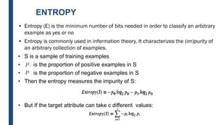
17. ENTROPY - EXAMPLE
• Entropy([29+, 35-]) = - (29/64) log2(29/64) - (35/64) log2(35/64)
=0.99

18. INFORMATION GAIN
• Gain(S,A) = expected reduction in entropy by
partitioning the examples according to the attribute A
• Here values(A) is the set of all possible values for attribute A, sv
is the subset of S for which atribute A has value v
• Information gain measures the expected reduction in Entropy
• It measures the effectiveness of the attribute in classifying the
training data

19. An Illustrative Example

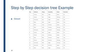
20. DECISION TREE LEARNING
■ Let’s Try an Example!
■ Let
– E([X+,Y-]) represent that there are X positive training elements
and Y negative elements.
■ Therefore the Entropy for the training data, E(S), can be
represented as E([9+,5-]) because of the 14 training examples 9 of
them are yes and 5 of them are no.

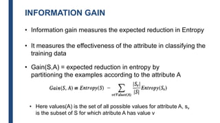
21. DECISION TREE LEARNING:
A SIMPLE EXAMPLE
■ Let’s start off by calculating the Entropy of the Training Set.
■ E(S) = E([9+,5-]) = (-9/14 log2 9/14) + (-5/14 log2 5/14)
■ = 0.94
■ Next we will need to calculate the information gain G(S,A) for
each attribute A where A is taken from the set {Outlook,
Temperature, Humidity, Wind}.

22. DECISION TREE LEARNING:
A SIMPLE EXAMPLE
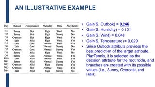
■ The information gain for Outlook is:
– Gain(S,Outlook) = E(S) – [5/14 * E(Outlook=sunny) + 4/14 *
E(Outlook = overcast) + 5/14 * E(Outlook=rain)]
– Gain(S,Outlook) = E([9+,5-]) – [5/14*E(2+,3-) +
4/14*E([4+,0]) + 5/14*E([3+,2-])]
– Gain(S,Outlook) = 0.94 – [5/14*0.971 + 4/14*0.0 +
5/14*0.971]
– Gain(S,Outlook) = 0.246

23. DECISION TREE LEARNING:
A SIMPLE EXAMPLE
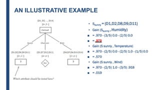
■ Gain(S,Temperature) = 0.94 – [4/14*E(Temperature=hot) +
6/14*E(Temperature=mild) +
4/14*E(Temperature=cool)]
■ Gain(S,Temperature) = 0.94 – [4/14*E([2+,2-]) + 6/14*E([4+,2-]) +
4/14*E([3+,1-])]
■ Gain(S,Temperature) = 0.94 – [4/14 + 6/14*0.918 + 4/14*0.811]
■ Gain(S,Temperature) = 0.029

24. DECISION TREE LEARNING:
A SIMPLE EXAMPLE
■ Gain(S,Humidity) = 0.94 – [7/14*E(Humidity=high) +
7/14*E(Humidity=normal)]
■ Gain(S,Humidity = 0.94 – [7/14*E([3+,4-]) + 7/14*E([6+,1-])]
■ Gain(S,Humidity = 0.94 – [7/14*0.985 + 7/14*0.592]
■ Gain(S,Humidity) = 0.1515

25. DECISION TREE LEARNING:
A SIMPLE EXAMPLE
■ G(S,Wind) = 0.94 – [8/14*0.811 + 6/14*1.00]
■ G(S,Wind) = 0.048

26. AN ILLUSTRATIVE EXAMPLE
• Gain(S, Outlook) = 0.246
• Gain(S, Humidity) = 0.151
• Gain(S, Wind) = 0.048
• Gain(S, Temperature) = 0.029
• Since Outlook attribute provides the
best prediction of the target attribute,
PlayTennis, it is selected as the
decision attribute for the root node, and
branches are created with its possible
values (i.e., Sunny, Overcast, and
Rain).

27. AN ILLUSTRATIVE EXAMPLE
• Ssunny = {D1,D2,D8,D9,D11}
• Gain (Ssunny , Humidity)
■ = .970 - (3/5) 0.0 - (2/5) 0.0
■ = .970
• Gain (S sunny , Temperature)
■ = .970 - (2/5) 0.0 - (2/5) 1.0 - (1/5) 0.0
■ = .570
• Gain (S sunny , Wind)
• Ssunny = {D1,D2,D8,D9,D11}
• Gain (Ssunny , Humidity)
■ = .970 - (3/5) 0.0 - (2/5) 0.0
■ = .970
• Gain (S sunny , Temperature)
■ = .970 - (2/5) 0.0 - (2/5) 1.0 - (1/5) 0.0
■ = .570
• Gain (S sunny , Wind)
■ = .970 - (2/5) 1.0 - (3/5) .918
■ = .019

28. FINAL DECISION TREE :

29. Classification And Regression Trees
(CART)
■ CART uses GINI index to construct the decision tree
■ We need to compute the best splitting attribute and the best split subset i in the
chosen attribute.
■ Higher GINI value, higher is the homogeneity of the instances.
29

30. Step by Step decision tree Example
■ Dataset
30

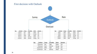
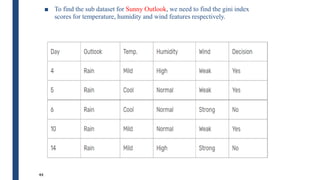
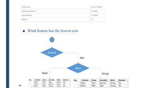
31. 31
■ Outlook is the feature with the values: sunny, overcast, rainy
■ Summary of Outlook is given by



j
t
j
p
t
GINI 2
)]
|
(
[
1
)
(



k
i
i
split i
GINI
n
n
GINI
1
)
(

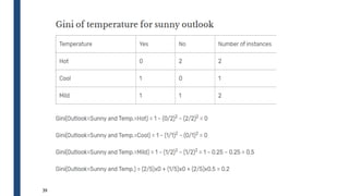
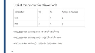
32. ■ Temperature is the feature with the values: Hot, cold, mild
■ Summary of Temperature is given by
32



j
t
j
p
t
GINI 2
)]
|
(
[
1
)
(



k
i
i
split i
GINI
n
n
GINI
1
)
(

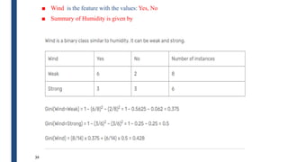
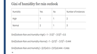
33. ■ Humidity is the feature with the values: High, Normal
■ Summary of Humidity is given by
33



j
t
j
p
t
GINI 2
)]
|
(
[
1
)
(



k
i
i
split i
GINI
n
n
GINI
1
)
(

34. ■ Wind is the feature with the values: Yes, No
■ Summary of Humidity is given by
34

35. ■ Choose the feature with lowest Gini index cost as the root node.
■ Outlook has the lowest cost.
35

36. First decision with Outlook
36

37. ■ Overcast leaf has only yes decisions. This means that overcast becomes the
leaf node.
37

38. ■ To find the sub dataset for Sunny Outlook, we need to find the gini index scores
for temperature, humidity and wind features respectively.
38

39. 39

40. 40

41. 41

42. Humidity has lowest Gini index:
42

43. ■ Decision is always no for high humidity and sunny outlook and decision
will always be yes for normal humidity and sunny outlook.
43

44. ■ To find the sub dataset for Sunny Outlook, we need to find the gini index
scores for temperature, humidity and wind features respectively.
44

45. 45

46. 46

47. 47

48. ■ Wind feature has the lowest cost
48

49. ■ Decision is always yes when wind is weak. And decision is always no if
wind is strong.
■ With this Decision tree is complete.
49

50. Regression trees
■ Procedure for Constructing Decision trees
– Compute standard deviation for each attribute with respect to target
attribute
– Compute SD for number of data instances of each distinct value of an
attribute.
– Compute weighted standard deviation for each attribute.
– Compute standard deviation reduction by subtracting standard
deviation for each attribute from standard deviation of each attribute.
– Choose the attribute with a higher standard deviation reduction as the
best split attribute.
– The best split attribute is placed as the root node.
■ Follow the steps from the Text Book
50