Download as PDF, PPTX


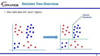
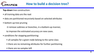
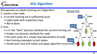
![21
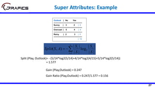
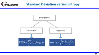
Selecting The Root Node
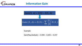
[2+, 3-]
Outlook
Sunny Rain
[3+, 2-]
Play=[9+,5-]
E=0.940
Gain(Play,Outlook) = 0.940 –
((5/14)*0.971 + (4/14)*0.0 +
(5/14)*0.971)= 0.247
E=0.971 E=0.971
Overcast
[4+, 0-]
E=0.0
Temp
Hot Cool
[2+, 2-] [3+, 1-]
Play=[9+,5-]
E=0.940
Gain(Play,Temp) = 0.940 –
((4/14)*1.0 + (6/14)*0.918 +
(4/14)*0.811)= 0.029
E=1.0 E=0.811
Mild
[4+, 2-]
E=0.918](https://image.slidesharecdn.com/decisiontrees-200321113210/85/Decision-trees-22-320.jpg)
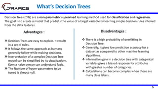
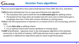
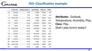
![22
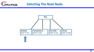
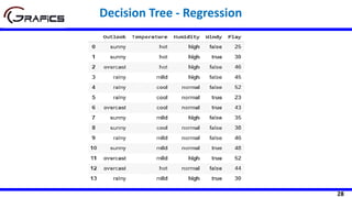
Humidity
High Normal
[3+, 4-] [6+, 1-]
Play=[9+,5-]
E=0.940
Gain(Play,Humidity) = 0.940 – ((7/14)*0.985
+ (7/14)*0.592)= 0.152
E=0.985 E=0.592
Windy
false true
[6+, 2-] [3+, 3-]
Play=[9+,5-]
E=0.940
Gain(Play,Wind) = 0.940 – ((8/14)*0.811 + (6/14)*1.0)
= 0.048
E=0.811 E=1.0
Selecting The Root Node](https://image.slidesharecdn.com/decisiontrees-200321113210/85/Decision-trees-23-320.jpg)

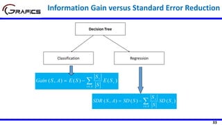
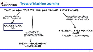
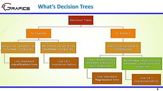
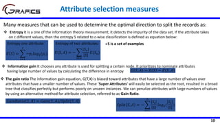
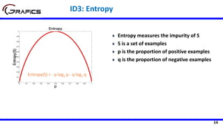
![34
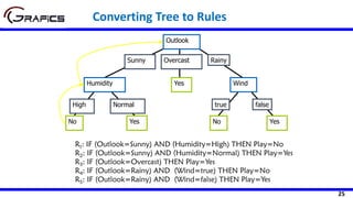
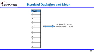
Selecting The Root Node
SDR(Play,Outlook) = 9.32 - ((5/14)*7.78
+ (4/14)*3.49 + (5/14)*10.87)
= 1.662
Outlook
Sunny Rain
[5] [5]
Play=[14]
SD=9.32
SD=7.78 SD=10.87
Overcast
[4]
SD=3.49
Temp
Hot Cool
[4] [4]
Play=[14]
SD=9.32
SD=8.95 SD=10.51
Mild
[6]
SD=7.65
SDR(Play,Temp) =9.32 - ((4/14)*8.95 +
(6/14)*7.65 + (4/14)*10.51)
=0.481](https://image.slidesharecdn.com/decisiontrees-200321113210/85/Decision-trees-35-320.jpg)
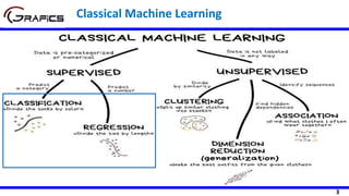
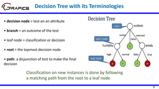
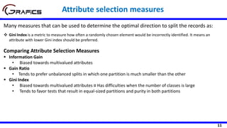
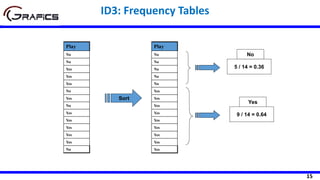
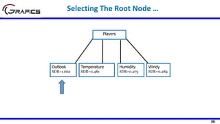
![35
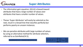
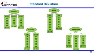
Humidity
High Normal
[7] [7]
Play=[14]
SD= 9.32
SDR(Play,Humidity) =9.32 - ((7/14)*9.36
+ (7/14)*8.73)=0.275
SD=9.36 SD=8.73
Selecting The Root Node …
Windy
Weak Strong
[8] [6]
Play=[14]
SD= 9.32
SD=7.87 SD=10.59
SDR(Play,Humidity) =9.32 - ((8/14)*7.87
+ (6/14)*10.59)=0.284](https://image.slidesharecdn.com/decisiontrees-200321113210/85/Decision-trees-36-320.jpg)
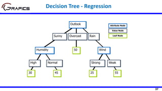
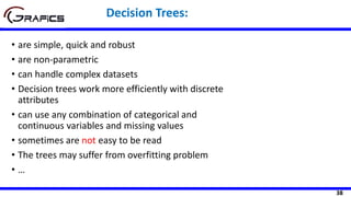

The document discusses decision tree models in machine learning. It begins by defining key terms like decision nodes, branches, and leaf nodes. It then explains how decision trees are built in a top-down manner by recursively splitting the training data based on selected attributes. The document also covers different algorithms for building decision trees like ID3, C4.5, and CART. It discusses measures used for attribute selection like information gain, gain ratio, and Gini index. Finally, it provides an example of how to build a decision tree to classify whether to play tennis based on weather attributes.