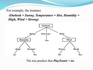
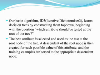
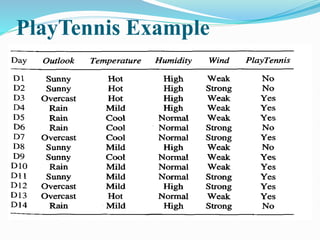
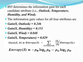
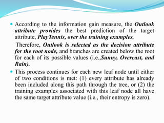
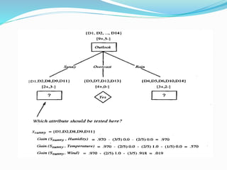
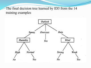
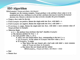
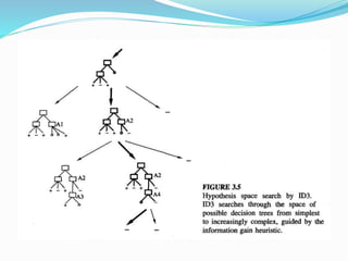
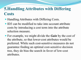
The document discusses decision tree learning and the ID3 algorithm. It begins by introducing decision trees and how they are used to classify instances by sorting them from the root node to a leaf node. It then discusses how ID3 builds decision trees in a top-down greedy manner by selecting the attribute that best splits the data at each node based on information gain. The document also covers issues like overfitting, handling continuous attributes, and pruning decision trees.

1. K LAKSHMI SRAVANI
Asst Prof

2. INTRODUCTION
 Decision tree learning is a method for approximating
discrete-valued target functions, in which the learned
function is represented by a decision tree.
 Learned trees can also be re-represented as sets of if-then
rules to improve human readability

3. DECISION TREE
REPRESENTATION
 Decision trees classify instances by sorting them down the
tree from the root to some leaf node, which provides the
classification of the instance.
 Each node in the tree specifies a test of some attribute of
the instance, and each branch descending from that node
corresponds to one of the possible values for this attribute.

4. Decision tree for the concept
PlayTennis.
Decision tree corresponds to the expression
(Outlook = Sunny Humidity = Normal)
V (Outlook = Overcast)
V (Outlook = Rain Wind = Weak)

5. For example, the instance
(Outlook = Sunny, Temperature = Hot, Humidity =
High, Wind = Strong)
The tree predicts that PlayTennis = no

6. APPROPRIATE PROBLEMS FOR DECISION
TREE LEARNING
 Instances are represented by attribute-value pairs.
 The target function has discrete output values.
 Disjunctive descriptions may be required.
 The training data may contain errors.
 The training data may contain missing attribute values.

7. APPLICATIONS
 Many practical problems have been found to fit these
characteristics.
 Decision tree learning has therefore been applied to
problems such as learning to classify medical patients by
their disease, equipment malfunctions by their cause, and
loan applicants by their likelihood of defaulting on
payments.
 Such problems, in which the task is to classify examples
into one of a discrete set of possible categories, are often
referred to as classification problems.

8. THE BASIC DECISION TREE
LEARNING ALGORITHM
 Most algorithms that have been developed for learning
decision trees are variations on a core algorithm that
employs a top-down, greedy search through the space of
possible decision trees.
 This approach is exemplified by the ID3(Iterative
Dichotomiser3) algorithm (Quinlan 1986) and its
successor C4.5 (Quinlan 1993).

9.  Our basic algorithm, ID3(Iterative Dichotomiser3), learns
decision trees by constructing them topdown, beginning
with the question "which attribute should be tested at the
root of the tree?”
 The best attribute is selected and used as the test at the
root node of the tree. A descendant of the root node is then
created for each possible value of this attribute, and the
training examples are sorted to the appropriate descendant
node.

10. The entire process is then repeated using
the training examples associated with
each descendant node to select the best
attribute to test at that point in the tree.
This forms a greedy search for an
acceptable decision tree, in which the
algorithm never backtracks to reconsider
earlier choices.

11. Which Attribute Is the Best
Classifier?
 The statistical property, called information gain, that
measures how well a given attribute separates the training
examples according to their target classification.
 ID3(Iterative Dichotomiser3) uses this information gain
measure to select among the candidate attributes at each
step while growing the tree.

12. ENTROPY MEASURES HOMOGENEITY OF
EXAMPLES
 To define Information Gain, first need to know about the
information theory called entropy S.
 It characterizes the impurity of an arbitrary collection of
examples.

13.  In given collection ,containing positive and negative
examples of some target concept, the entropy of S relative
to this boolean classification is
 where p is the proportion of positive examples in S and p
is the proportion of negative examples in S. In all
calculations involving entropy we define 0 log 0 to be 0.

14.  For example, if all members are positive
(p+ve = I), then p-ve is 0, and
Entropy(S) =-1 . log2(1) - 0 . log2 0
= -1 . 0 - 0 . log2 0 = 0.
 Note the entropy is 1 when the collection contains an
equal number of positive and negative examples. If the
collection contains unequal numbers of positive and
negative examples, the entropy is between 0 and 1.

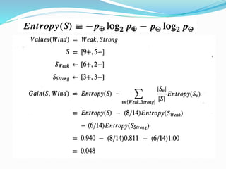
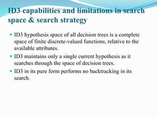
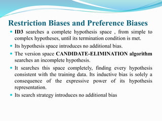
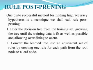
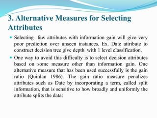
15.  suppose S is a collection of 14 examples of some Boolean
concept, including 9 positive and 5 negative examples (we
adopt the notation[9+, 5-] to summarize such a sample of
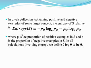
data). Then the entropy of S relative to
this Boolean classification is

16. The entropy function relative to a boolean
classification, as the proportion, p+ve, of
positive examples varies p-ve between 0 and 1.

17.  More generally, if the target attribute can take on c
different values, then the entropy of S relative to this c-
wise classification is defined as
where pi is the proportion of S belonging to class i.
 Note the logarithm is still base 2 because entropy is a
measure of the expected encoding length measured in bits.
Note also that if the target attribute can take on c possible
values, the entropy can be as large as log2 c.

18. INFORMATION GAIN MEASURES THE
EXPECTED REDUCTION IN ENTROPY
 The entropy as a measure of the impurity in a collection of
training examples, we can now define a measure of the
effectiveness of an attribute in classifying the training data.

19.  The Information gain, is simply the expected reduction in
entropy caused by partitioning the examples according to
this attribute. More precisely, the information gain,
Gain(S, A) of an attribute A, relative to a collection of
examples S, is defined as
 where Values(A) is the set of all possible values for
attribute A, and S, is the subset of S for which attribute A
has value v

20. PlayTennis Example

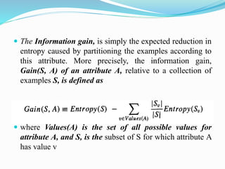
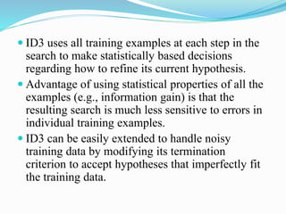
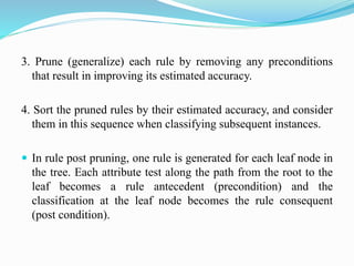
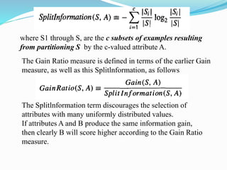
21.  Gain(S, A) gives the expected reduction in entropy caused
by knowing the value of attribute.
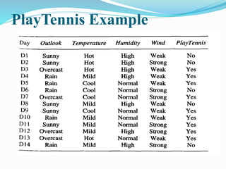
 For example, suppose S is a collection of training-example
days described by attributes including Wind, which can
have the values Weak or Strong. As before, assume S is a
collection containing 14 examples, [9+, 5-]. Of these 14
examples,
 suppose 6 of the positive and 2 of the negative examples
have Wind = Weak, and the remainder have Wind =
Strong. The information gain due to sorting the original 14
examples by the attribute Wind may then be calculated as

24. PlayTennis Example

25.  ID3 determines the information gain for each
candidate attribute (i.e., Outlook, Temperature,
Humidity, and Wind).
 The information gain values for all four attributes are
 Gain(S, Outlook) = 0.246
 Gain(S, Humidity) = 0.151
 Gain(S, Wind) = 0.048
 Gain(S, Temperature) = 0.029

26.  According to the information gain measure, the Outlook
attribute provides the best prediction of the target
attribute, PlayTennis, over the training examples.
Therefore, Outlook is selected as the decision attribute
for the root node, and branches are created below the root
for each of its possible values (i.e.,Sunny, Overcast, and
Rain).
 This process continues for each new leaf node until either
of two conditions is met: (1) every attribute has already
been included along this path through the tree, or (2) the
training examples associated with this leaf node all have
the same target attribute value (i.e., their entropy is zero).

28. The final decision tree learned by ID3 from the 14
training examples

29. ID3 Algorithm

30. HYPOTHESIS SPACE SEARCH IN
DECISION TREE LEARNING
 ID3 can be characterized as searching a space of
hypotheses for one that fits the training examples.
 The hypothesis space searched by ID3 is the set of
possible decision trees.
 ID3 performs a simple-to complex, hill-climbing search
through this hypothesis space, beginning with the empty
tree, then considering progressively more elaborate
hypotheses in search of a decision tree that correctly
classifies the training data.
 The evaluation function that guides this hill-climbing
search is the information gain measure.

32. ID3 capabilities and limitations in search
space & search strategy
 ID3 hypothesis space of all decision trees is a complete
space of finite discrete-valued functions, relative to the
available attributes.
 ID3 maintains only a single current hypothesis as it
searches through the space of decision trees.
 ID3 in its pure form performs no backtracking in its
search.

33.  ID3 uses all training examples at each step in the
search to make statistically based decisions
regarding how to refine its current hypothesis.
 Advantage of using statistical properties of all the
examples (e.g., information gain) is that the
resulting search is much less sensitive to errors in
individual training examples.
 ID3 can be easily extended to handle noisy
training data by modifying its termination
criterion to accept hypotheses that imperfectly fit
the training data.

34. INDUCTIVE BIAS IN DECISION TREE
LEARNING
 Inductive bias is the set of assumptions that,
together with the training data, deductively justify
the classifications assigned by the learner to future
instances.
 Describing the inductive bias of ID3 therefore
consists of describing the basis by which it
chooses one of these consistent hypotheses over
the all possible decision trees.

35.  Approximate inductive bias of ID3: Shorter trees
are preferred over larger trees it uses
BFS(Breadth First Search).
 A closer approximation to the inductive bias of
ID3: Trees that place high information gain
attributes close to the root are preferred over those
that do not.

36. Restriction Biases and Preference Biases
 ID3 searches a complete hypothesis space , from simple to
complex hypotheses, until its termination condition is met.
 Its hypothesis space introduces no additional bias.
 The version space CANDIDATE-ELIMINATION algorithm
searches an incomplete hypothesis.
 It searches this space completely, finding every hypothesis
consistent with the training data. Its inductive bias is solely a
consequence of the expressive power of its hypothesis
representation.
 Its search strategy introduces no additional bias

37.  The inductive bias of ID3 follows from its search strategy,
whereas the inductive bias of the CANDIDATE-
ELIMINATION algorithm follows from the definition of its
search space.
 The inductive bias of ID3 is thus a preference for certain
hypotheses over others (e.g., for shorter hypotheses). This form
of bias is typically called a preference bias (or, a search bias).
 In contrast, the bias of the CANDIDAT-EELIMINATION
algorithm is in the form of a categorical restriction on the set
of hypotheses considered. This form of bias is typically called a
restriction bias (or, a language bias).

38. Why Prefer Short Hypotheses?
 William of Occam was one of the first to discuss the
question, around the year 1320, so this bias often goes by
the name of Occam's razor.
 Occam's razor: “Prefer the simplest hypothesis that fits
the data”.
 It is the problem solving principle that the simplest
solution tends to be the right one.
 When presented with competing hypothesis to solve a
problem, one should select a solution with the fewest
assumptions.
 Shorter hypothesis fits the training data which are less
likely to be consist training data.

39. ISSUES IN DECISION TREE LEARNING
1.Avoiding Over fitting the Data
Reduced error pruning.
Rule post –pruning.
2. Incorporating Continuous-Valued Attributes.
3. Alternatively Measures for Selecting Attributes.
4. Handling Training Examples with Missing Attributes
Values.
5. Handling Attributes with Differing Costs.

40. ISSUES IN DECISION TREE LEARNING
Avoiding Overfitting the Data:
Definition: Given a hypothesis space H, a
hypothesis h H is said to overfit the training data
if there exists some alternative hypothesis h' H,
such that h has smaller error than h' over the
training examples, but h' has a smaller error than h
over the entire distribution of instances.

41. The impact of overfitting in a typical application of
decision tree learning. In this case, the ID3 algorithm is
applied to the task of learning which medical patients
have a form of diabetes.

42. There are several approaches to avoiding over fitting in
decision tree learning.
These can be grouped into two classes:
1.Approaches that stop growing the tree earlier, before it
reaches the point where it perfectly classifies the
training data.
2. Approaches that allow the tree to overfit the data, and
then post-prune the tree.

43.  To determine the correct final tree size. Approaches include:
 Use a separate set of examples, distinct from the training examples, to
evaluate the utility of post-pruning nodes from the tree.
 Use all the available data for training, but apply a statistical test to estimate
whether expanding (or pruning) a particular node is likely to produce an
improvement beyond the training set. For example, Quinlan (1986) uses a
chi-square test to estimate whether further expanding a node is likely to
improve performance over the entire instance distribution, or only on the
current sample of training data.
 Use an explicit measure of the complexity for encoding the training
examples and the decision tree, halting growth of the tree when this
encoding size is minimized. This approach, based on a heuristic called the
Minimum Description Length principle, as well as in Quinlan and Rivest
(1989) and Mehta et al. (199.5).

44.  The available data are separated into 2 sets of examples: a
training set, which is used to form the learned hypothesis, and
a separate validation set, which is used to evaluate the accuracy
of this hypothesis over subsequent data and , in particular, to
evaluate the impact of pruning this hypothesis.
 Withhold one-third of the available ex. for the validation set,
using the other two-thirds for training.

45. REDUCED ERROR PRUNING
 One approach, called reduced-error pruning (Quinlan
1987), is to consider each of the decision
nodes in the tree to be candidates for pruning. Pruning a
decision node consists of removing the subtree rooted at
that node, making it a leaf node, and assigning it the most
common classification of the training examples affiliated
with that node.
 Nodes are removed only if the resulting pruned tree
performs no worse than-the original over the validation
set.

46. As pruning proceeds, the number of nodes is reduced and accuracy over
the test set increases. Here, the available data has been split into three
subsets: the training examples, the validation examples used for pruning
the tree, and a set of test examples used to provide an unbiased estimate
of accuracy over future unseen examples.

47.  The major drawback of this approach is that when
data is limited, withholding part of it for the
validation set reduces even further the number of
examples available for training.

48. RULE POST-PRUNING
One quite successful method for finding high accuracy
hypotheses is a technique we shall call rule post-
pruning.
1. Infer the decision tree from the training set, growing
the tree until the training data is fit as well as possible
and allowing over-fitting to occur.
2. Convert the learned tree into an equivalent set of
rules by creating one rule for each path from the root
node to a leaf node.

49. 3. Prune (generalize) each rule by removing any preconditions
that result in improving its estimated accuracy.
4. Sort the pruned rules by their estimated accuracy, and consider
them in this sequence when classifying subsequent instances.
 In rule post pruning, one rule is generated for each leaf node in
the tree. Each attribute test along the path from the root to the
leaf becomes a rule antecedent (precondition) and the
classification at the leaf node becomes the rule consequent
(post condition).

50. Convert the decision tree to rules before
pruning has 3 main advantages.
 Converting to rules allows distinguishing among the different
contexts in which a decision node is used. Because each
distinct path through the decision tree node produces a distinct
rule, the pruning decision regarding that attribute test can be
made differently for each path. In contrast, if the tree itself
were pruned, the only two choices would be to remove the
decision node completely, or to retain it in its original form.
 Converting to rules removes the distinction between attribute
tests that occur near the root of the tree and those that occur
near the leaves. Thus, we avoid messy bookkeeping issues such
as how to reorganize the tree if the root node is pruned while
retaining part of the subtree below this test.
 Converting to rules improves readability. Rules are often easier
for to understand.

51. 2.Incorporating Continuous-Valued Attributes
ID3 restrictions to attributes:
 First, the target attribute whose value is predicted by the
learned tree must be discrete valued. Second, the attributes
tested in the decision nodes of the tree must also be discrete
valued.
 Dynamically defining new discrete valued attributes that
partition the continuous attribute value into a discrete set of
intervals.
 A that is continuous-valued, the algorithm can dynamically
create a new boolean attribute A, that is true if A < c and false
otherwise.

52.  PlayTennis Ex. With possible temperatures.
 These candidate thresholds can then be evaluated by computing the
information gain associated with each.
 In the current example, there are two candidate thresholds,
corresponding to the values of Temperature at which the value of
PlayTennis changes: (48 + 60)/2 and (80 + 90)/2.
 The information gain can then be computed for each of the candidate
attributes, (Temperature >54) and (Temperature > 85 )the best can
be selected (Temperature > 54). This dynamically created Boolean
attribute can then compete with the other discrete-valued candidate
attributes available for growing the decision tree.

53. 3. Alternative Measures for Selecting
Attributes
 Selecting few attributes with information gain will give very
poor prediction over unseen instances. Ex. Date attribute to
construct decision tree give depth with 1 level classification.
 One way to avoid this difficulty is to select decision attributes
based on some measure other than information gain. One
alternative measure that has been used successfully is the gain
ratio (Quinlan 1986). The gain ratio measure penalizes
attributes such as Date by incorporating a term, called split
information, that is sensitive to how broadly and uniformly the
attribute splits the data:

54. where S1 through S, are the c subsets of examples resulting
from partitioning S by the c-valued attribute A.
The Gain Ratio measure is defined in terms of the earlier Gain
measure, as well as this Splitlnformation, as follows
The Splitlnformation term discourages the selection of
attributes with many uniformly distributed values.
If attributes A and B produce the same information gain,
then clearly B will score higher according to the Gain Ratio
measure.

55. 4.Handling Training Examples with
Missing Attribute Values
 Consider the situation in which Gain(S, A) is to be calculated at node n
in the decision tree to evaluate whether the attribute A is the best
attribute to test at this decision node. Suppose that (x, c(x)) is one of
the training examples in S and that the value A(x) is unknown.
 One strategy for dealing with the missing attribute value is to assign it
the value that is most common among training examples at node n.
Alternatively, we might assign it the most common value among
examples at node n that have the classification c(x). The elaborated
training example using this estimated value for A(x) can then be used
directly by the existing decision tree learning algorithm. This strategy
is examined by Mingers (1989a).

56.  A second, more complex procedure is to assign a
probability to each of the possible values of A
rather than simply assigning the most common
value to A(x).
 These probabilities can be estimated again based
on the observed frequencies of the various values
for A among the examples at node n.

57. 5.Handling Attributes with Differing
Costs
 Handling Attributes with Differing Costs.
 ID3 can be modified to take into account attribute
costs by introducing a cost term into the attribute
selection measure.
 For example, we might divide the Gain by the cost of
the attribute, so that lower-cost attributes would be
preferred. While such cost-sensitive measures do not
guarantee finding an optimal cost-sensitive decision
tree, they do bias the search in favor of low-cost
attributes.

58.  Attribute cost is measured by the number of seconds
required to obtain the attribute value by positioning
and operating the sonar. They demonstrate that more
efficient recognition strategies are learned, without
sacrificing classification accuracy, by replacing the
information gain attribute selection measure by the
following measure

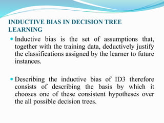
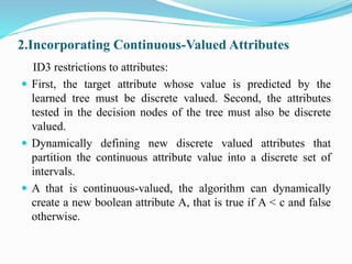
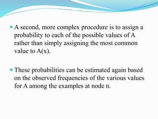
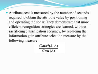
59.  Nunez (1988) describes a related approach and its
application to learning medical diagnosis rules. Here the
attributes are different symptoms and laboratory tests with
differing costs. His system uses a somewhat different
attribute selection measure
 where w [0, 1] is a constant that determines the relative
importance of cost versus information gain. Nunez (1991)
presents an empirical comparison of these two approaches
over a range of tasks.