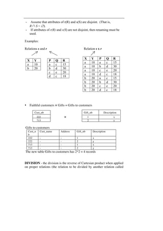
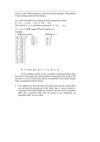
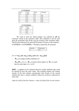
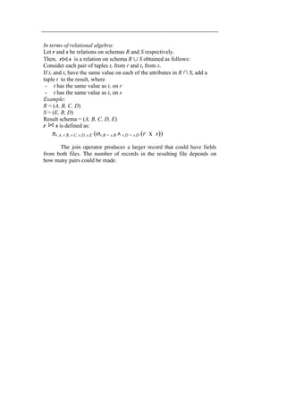
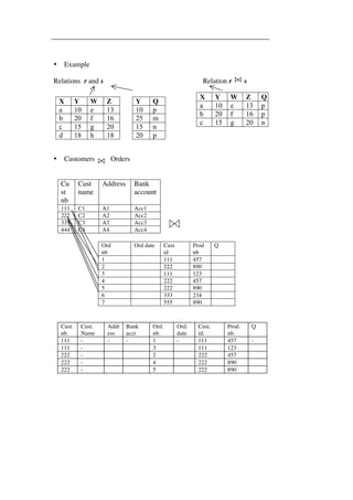
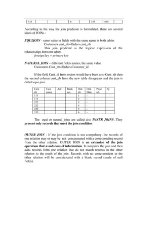
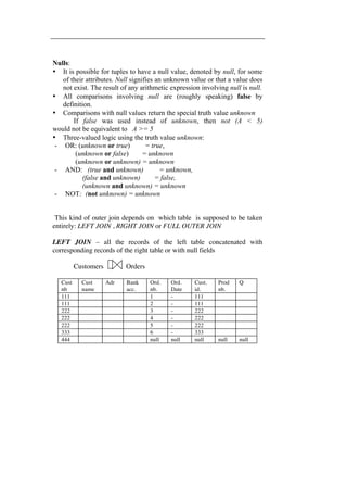
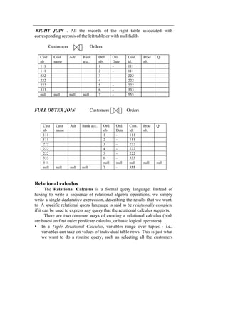
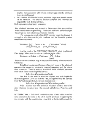
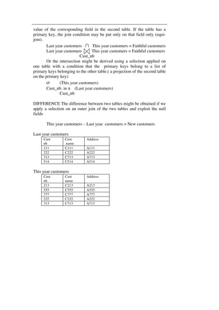
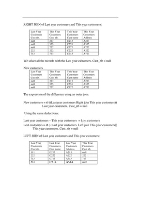
SlideShare a Scribd company logo
DATA MODELS 
A model is a representation of "real world" objects and events, and 
their associations. It concentrates on the essential, inherent aspects of an 
organization and ignores the accidental properties. Actually, there isn't 
really a data model "thing". Data models are abstractions, often times 
mathematical algorithms and concepts. You cannot really touch a data 
model. But nevertheless, they are very useful. A data model attempts to 
represent the data requirements of the organization, or the part of the 
organization that you wish to model. It should provide the basic concepts 
and notations that will allow database designers and end-users to 
communicate their understanding of the organizational data 
unambiguously and accurately. The purpose of a data model is to represent 
data and to make the data understandable. 
A data model consists of a collection of tools for describing: data, 
data relationships, data semantics and data constraints 
Data model - an integrated collection of concepts for describing 
data, relationships between data, and constraints on the data used by 
an organization. 
A data model can be thought of as comprising three components: 
• a structural part, consisting of a set of rules that define how a 
database is to be constructed; 
• a manipulative part, defining the types of operations that are 
allowed on the data (updating, retrieving data or changing the 
structure of the database) 
• possibly a set of integrity rules, which ensures that the data is 
accurate 
Thus, essentially a data model is a "description" of both a container 
for data and a methodology for storing and retrieving data from that 
container. The analysis and design of data models has been the 
cornerstone of the evolution of databases. As models have advanced so 
has database efficiency. 
The main feature that differentiates a database from a collection of 
traditional files is the existence of relationships between records regarding 
objects or facts that had something in common. For instance, the record 
that preserve data on a specific customer is related to records that store
data on the orders send by that customer and each order is related to 
records that describe the products mentioned in order lines. On the other 
side, more customers’ records may be related also to the record that holds 
data on their sales agent. This complex set of relationships once frozen in 
the database might be exploited to retrieve initial data in less time and 
with considerable less programming effort. 
The implementation of relationships is a technological matter 
leading to the different database models emerged in the last 30 years. The 
first attempt was to realize relationships between records at physical level. 
The most known physical relationships are pointers - extra fields added to 
the record and containing the address of the related record. The related 
record could be accessed directly by making use of the pointer. 
The pointer mechanism once set up, different data base models were 
invented according to the relationships pattern. Among them, the 
hierarchical data base model and the network database model, the two 
most commonly used database models before the 1980's. 
HIERARCHICAL DATABASE MODEL 
As its name implies, the Hierarchical Database Model defines 
hierarchically - arranged data. Perhaps the most intuitive way to visualize 
this type of relationship is by visualizing an upside down tree of data. In 
this tree, a single table acts as the "root" of the database from which other 
tables "branch" out. The hierarchical database model use a tree pattern in 
implementing relationships between records depicting different objects 
Relationships in such a system are thought of in terms of children 
and parents such that a child may only have one parent but a parent can 
have multiple children. Parents and children are tied together by links 
called "pointers". A parent will have a list of pointers to each of their 
children. 
This child/parent rule assures that data is systematically accessible. 
To get to a low-level table, you start at the root and work your way down 
through the tree until you reach your target. One serious problem is that 
the user must know how the tree is structured in order to find anything.
Sales agent 1122 
Customer 5543 Customer 6689 Customer 1122 
order 123 
order 145 
product 144 product 553 product 337 
Fig. 3.1. The hierarchical data model 
The sales agent’s record at the root of the tree has pointers to 
records of all customers he represents, each customer record has pointers 
to all his orders records and each order record has pointers to all the 
ordered products. The tree expands at lower levels with every new order 
sent by a customer. The structure needs a lot of extra fields for each record 
to accommodate the new emerging vertical relationships. 
The hierarchical model however, is much more efficient than the 
flat-file model because there is not as much need for redundant data. If a 
change in the data is necessary, the change might only need to be 
processed once. As we mentioned before, this flat file database would 
store an excessive amount of redundant data. If we implemented this in a 
hierarchical database model, we would get much less redundant data. 
Consider the following hierarchical database scheme: 
However, the hierarchical database model has some serious 
problems. For one, you cannot add a record to a child table until it has 
already been incorporated into the parent table (for instance, you can't add 
a new customer if that customer is not represented by a sale agent). Also, 
the hierarchical database model still creates repetition of data within the 
database. Redundancy would occur because hierarchical databases handle 
one-to-many relationships well but do not handle many-to-many 
relationships well. This is because a child may only have one parent. 
However, in many cases the child must be related to more than one parent.
Though this problem can be solved with multiple databases 
creating logical links between children, the fix is very kludgy and 
awkward. 
NETWORK DATABASE MODEL 
In many ways, the Network Database model was designed to solve 
some of the more serious problems with the Hierarchical Database Model. 
Specifically, the Network model solves the problem of data redundancy by 
representing relationships in terms of sets rather than hierarchy. The 
model had its origins in the Conference on Data Systems Languages 
(CODASYL) which had created the Data Base Task Group to explore and 
design a method to replace the hierarchical model. 
The network model is very similar to the hierarchical model. In 
fact, the hierarchical model is a subset of the network model. However, 
instead of using a single-parent tree hierarchy, the network model uses set 
theory to provide a tree-like hierarchy with the exception that child tables 
were allowed to have more than one parent. This allowed the network 
model to support many-to-many relationships. 
Visually, a Network Database looks like a hierarchical Database in 
that you can see it as a type of tree. However, in the case of a Network 
Database, the look is more like several trees which share branches. Thus, 
children can have multiple parents and parents can have multiple children. 
The records at each tree level are related by horizontal links and form a 
chained forward list that could be extended at the end of the chain with 
new emerging records 
Sales agent 1122 
Sales agent 2233 
Customer 5543 Customer 6689 Customer 1122 
order 123 order 145 
product 144 product 553 product 337 
Fig. 3.2. The network data model
The vertical relationships (between records depicting different 
entities) need only one pointer to reach the beginning of the chain of 
related records. The horizontal relationships (between similar records) 
need only one pointer to reach the next record in chain. An extra pointer 
could be added to indicate the previous record, providing backward 
chaining. The end of the record chain is indicated by a special stop value 
for the pointer. The network model can be expanded easier with new 
similar records at any level and the pointer number in each record remains 
the same. 
Nevertheless, though it was a dramatic improvement, the network 
model was far from perfect. Most profoundly, the model was difficult to 
implement and maintain. Most implementations of the network model 
were used by computer programmers rather than real users. What was 
needed was a simple model which could be used by real end users to solve 
real problems. 
Data accessing in data bases using physical pointers exploit the 
chaining mechanism to retrieve related records. Special software support 
must be provided for each database model to allow the user to extract data 
without being very much aware of the internal organization of the 
database. 
A major inconvenient of physical relationships is that they depend on 
the physical support of the database. Every time the database is 
transported from one media to another, the pointers' values must be 
updated. To overcome this inconvenient, a new technique in implementing 
the relationships was invented: logical relationships. 
The logical relationships are virtual relationships created between 
records on the basis of a common field. The records are related at retrieval 
time by matching records with the same value in the common field. At 
storage time, the records are stored in separate files and checked to meet 
relating criteria (values in the common fields to match existing values in 
virtually related files). 
Databases created with logical relationships store data easier but 
require a lot of special software support to retrieve it. Also, the virtual 
relationships lead to a lot of restrictions imposed to data at storage time to 
ensure that the new entered record is truly related to the rest of the data 
base.
THE RELATIONAL MODEL 
The relational model - which implements logical relationships 
between files in a database - was the first theoretically founded and well 
thought out data model first proposed by E.F. Codd in 1970. The model is 
based on branches of mathematics called set theory and predicate logic. 
The basic idea behind the relational model is that a database consists of a 
series of unordered tables (or relations) that can be manipulated using non-procedural 
operations that return tables. This model was in vast contrast to 
the more traditional database theories of the time that were much more 
complicated, less flexible and dependent on the physical storage methods 
of the data. It was the foundation of both database software and theoretical 
database research ever since. 
Relational data structure 
The relational data model is based on the structures and mathematics 
of relations. The term relation is a mathematical term which means a two-dimensional 
table which is not homogeneous in its rows, i.e. , the number 
of rows (unlike the number of columns) is not fixed. It is synonymous 
with the term table, thus the table is not a fixed structure like a matrix or 
an array which have fixed row and column dimensions, for the relation the 
total number of rows can grow and shrink according to need. 
In the relational model, we use relations to hold information about the 
objects we want to represent in the database. We represent a relation as a 
table in which the rows of the table correspond to individual records and 
the table columns correspond to attributes. A row is also known as a tuple 
(from quintuple, sextuple etc., a group of n elements is an n-tuple) and a 
column an attribute. Each attribute has unique name and although it isn't 
shown here the row order and column order are not significant. Each row 
must also be unique.
Example: Table Customers 
attributes (columns, fields) 
Every value within a given attribute must be of the same type and the 
collection of values for an attribute is known as a domain. A domain is 
the set of allowable values for one or more attributes. The domain concept 
is important because it allows us to define the meaning and source of 
values that attributes can hold. As a result, more information is available 
to the system and it can (theoretically) reject operations that don't make 
sense. 
Formally, given sets D1, D2, …. Dn a relation r is a subset of 
D1 x D2 x … x Dn 
Thus a relation is a set of n-tuples (a1, a2, …, an) where 
each ai ∈ Di 
Example: if 
Customer_id={1111,1253,2121,1555} 
Customer_name = {Jones, Smith, Curry, Lindsay} 
customer_city = {London, London, Manchester, Reading} 
balance = {500,200,600,300} 
Then r = {(1111,Jones, London, 500), 
(1253,Smith, London, 200), 
(2121,Curry, Manchester, 600), 
(1555,Lindsay, Reading, 300)} 
is a relation over customer_id x customer_name x customer-city x 
balance 
The relation has the following properties: 
tuples 
(rows,records) 
Customer_id Customer_name Customer_city Balance 
1111 Jones London 500 
1253 Smith London 200 
2121 Curry Manchester 600 
1555 Lindsay Reading 300
• Each entry in the table occurs only once (each row is unique). 
• Each column is named 
• All values of a given column are of the same type 
• Column order is immaterial 
• Row order is immaterial 
A relational database consists of tables that are appropriately 
structured. The appropriateness is obtained through the process of 
normalization. So, we can define a relational database as being a 
collection of normalized tables. 
A relational table has the following properties: 
• The table has a name that is distinct from all other tables in the 
database. 
• Each column has a distinct name. 
• The values of a column are all from the same domain. 
• The order of columns has no significance. 
• Each record is distinct; there are no duplicate records. 
• The order of records has no significance. 
• Each cell of the table (field) contains exactly one value (first 
normal form) 
The terminology of the relational model can be quite confusing. You 
can encounter terms like: 
- for relation: table or file 
- for tuple : row or record 
- for attribute : column or field 
Relational keys 
Each record in a table must be unique; that means we need to be 
able to identify a column (or combinations of columns) that provides 
uniqueness. 
Superkey - a column, or set of columns, that uniquely identifies a 
record within a table. 
Let K ⊆ R 
K is a superkey of R if values for K are sufficient to identify a unique tuple 
of each possible relation r(R)
by “possible r” we mean a relation r that could exist in the enterprise we 
are modeling. 
Example: {customer_id, customer_name} and 
{customer_id} 
are both superkeys of Customer, if no two customers can possibly have the 
same identification number. 
Since a superkey may contain additional columns that are not 
necessary for unique identification, we're interested in identifying 
superkeys that contain only the minimum number of columns necessary 
for unique identification. 
Candidate key - a superkey that contains only the minimum 
number of columns necessary for unique identification. 
K is a candidate key if K is minimal 
Example: {customer_id} is a candidate key for Customer, since it is a 
superkey (assuming no two customers can possibly have the same 
identification number), and no subset of it is a superkey. 
A candidate key has two properties: 
1. Uniqueness : in each record, the values of the candidate key uniquely 
identify the record 
2. Irreductibility (non-redundancy): no proper subset of the candidate 
key has the uniqueness property (no attribute in the key can be 
removed without destroying property 1) 
There may be more than one set of attributes which have both 
properties, these are candidate keys, one of which will be the primary key 
(the candidate key that is selected to identify uniquely records within the 
table) 
Thus, all columns (or combination of columns) in a table with unique 
values are referred to as candidate keys, from which the primary key must 
be drawn. All other candidate key columns are referred to as alternate 
keys. Keys can be simple or composite. A simple key is a key made up of 
one column, whereas a composite key is made up of two or more columns. 
The decision as to which candidate key is the primary one rests in your 
hands—there's no absolute rule as to which candidate key is best. Fabian 
Pascal, in his book SQL and Relational Basics, notes that the decision 
should be based upon the principles of minimality (choose the fewest 
columns necessary), stability (choose a key that seldom changes), and
simplicity/familiarity (choose a key that is both simple and familiar to 
users) 
Usually the word key refers to the primary key which implies that 
there are secondary keys. A secondary key is often used for speedy 
retrieval of rows from a table. 
There is another key called a foreign key - a column, or set of 
columns, within one table that matches the candidate key of some table. In 
other words, this is an attribute of a relation which identifies the primary 
key of another relation. A foreign key is a column in a table used to 
reference a primary key in another table. 
It is important that both foreign keys and the primary keys that are 
used to reference share a common meaning and draw their values from the 
same domain. The foreign key permits the association of multiple 
relations: 
TableA (A1, A2, A3) 
TableB (B1, B2, B3) 
TableC (A1,B1,C1) 
In TableC, attribute A1 is a foreign key of TableA and attribute B1 
is a foreign key of TableB. Foreign keys make it possible to resolve many-to- 
many associations between tables. 
One of the advantages of the database approach was control of data 
redundancy. This is an example of "controlled redundancy" -these 
common columns in different relations play an important role in modeling 
relationships. The foreign keys matching primary keys mechanism 
implements relationships between tables that share common fields.
The example used to illustrate the hierarchical and network database 
models is presented below in the relational approach: 
CUSTOMERS 
Customer_id 
Customer_name 
Customer_city 
Balance 
Creditlimit 
Slsanumb 
ORDERS 
Order_nb 
Order_date 
Customer_id 
PRODUCTS 
Prnumber 
Descrition 
MU 
Price 
Status 
Supply date 
Figure 3.3. The relational data model 
SALES 
AGENTS 
Slsanumb 
Slsaname 
Slasaaddr 
Totcomm 
Commrate 
ORDER LINES 
Order_nb 
Prnumber 
Quanyity 
The common convention for representing a description of a 
relational database is to give the name of each table, followed by the 
column names in parentheses. Normally, the primary key is underlined 
and foreign keys underlined with a dots line. In that example foreign keys 
are italic. 
SALES AGENTS(Slsanumb, Slsaname, Slasaaddr,Totcomm, Commrate) 
CUSTOMERS(Customer_id, Customer_name, Customer_city, Balance, 
Creditlimit, Slsanumb) 
ORDERS (Order_nb, Order_date, Customer_id) 
ORDER LINES (Order_nb, Prnumber, Quantity) 
PRODUCTS (Prnumber, Description, MU, Price, Status, Supply date) 
Besides the structure of data, the relational model also defines the 
means for data manipulation (relational algebra and relational calculus) 
and the means for specifying and enforcing data integrity (integrity 
constraints).
Relational integrity 
The relational model is very simple and efficient. Data are stored in 
tables that emulate the well-known file concept and duplicated columns in 
some tables that are to be related implement the virtual relationships. The 
model simplicity is balanced by a lot of rules that must be imposed to table 
structures and stored data to ensure the data precise retrieval. These rules 
are known as integrity rules and normal forms. 
Since every column (attribute) has an associated domain, there are 
constraints (called domain constraints) in the form of restrictions on the 
set of values allowed for the columns of tables. In addition, there are two 
important integrity rules, which are constraints or restrictions that apply to 
all instances of the database. 
NULLS 
Null represents a value for a column that is currently unknown or 
is not applicable for this record. A null can be taken to mean "unknown". 
It can also mean that a value is not applicable to a particular record, or it 
could just mean that no value has yet been supplied (missing). Nulls are a 
way to deal with incomplete or exceptional data. However, a null is not 
the same as a zero numeric value or a text string filled with spaces; zeros 
and spaces are values, but a null represents the absence of a value. 
Therefore, nulls should be treated differently from other values. 
INTEGRITY RULES 
The relational model defines several integrity rules that, while not 
part of the definition of the Normal Forms are nonetheless a necessary part 
of any relational database. There are two types of integrity rules: general 
and database-specific. 
General Integrity Rules 
The relational model specifies two general integrity rules. They are 
referred to as general rules, because they apply to all databases. They are: 
entity integrity and referential integrity. 
Entity integrity 
We know that a primary key is a minimal identifier that is used to 
identify records uniquely. This means that no subset of the primary key is 
sufficient to provide unique identification of records. If we allow a null
for any part of a primary key, we're implying that not all the columns are 
needed to distinguish between records, which contradicts the definition of 
the primary key. 
The first integrity rule applies to the primary keys of base tables: 
In a base table, no column of a primary key can be null 
A base table is a named table whose records are physically stored 
in the database (this in contrast to a view, a virtual table that does not 
actually exist in the database but is generated by the DBMS from the 
underlying tables whenever it's accessed). 
The entity integrity rule is very simple. It says that primary keys 
cannot contain null (missing) data. It's important to note that this rule 
applies to both simple and composite keys. For composite keys, none of 
the individual columns can be null. 
Referential integrity 
The second integrity rule applies to foreign keys. 
If a foreign key exists in a table, either the foreign key value must 
match a primary key value of some record in its home table or the 
foreign key value must be wholly null. 
The referential integrity rule says that the database must not contain 
any unmatched foreign key values. This implies that: 
• A row may not be added to a table with a foreign key unless the 
referenced value exists in the referenced table. 
• If the value in a table that's referenced by a foreign key is changed 
(or the entire row is deleted), the rows in the table with the foreign 
key must not be "orphaned." 
In general, there are three options available when a referenced primary 
key value changes or a row is deleted. The options are: 
• Disallow. The change is completely disallowed. 
• Cascade. For updates, the change is cascaded to all dependent 
tables. For deletions, the rows in all dependent tables are deleted. 
• Nullify. For deletions, the dependent foreign key values are set to 
Null 
Business rules 
All integrity constraints that do not fall under entity integrity or 
referential integrity are termed database-specific rules or business rules. 
These type of rules are specific to each database and come from the rules
of the business being modeled by the database. It is important to note that 
the enforcement of business rules is as important as the enforcement of the 
general integrity rules. Without the specification and enforcement of 
business rules, bad data will get in the database. 
Business rules are rules that define or constrain some aspect of the 
organization. Examples of business rules include domains, which 
constrain the values that a particular column can have, and the relational 
integrity rules. Another example is multiplicity, which defines the number 
of occurrences of one entity that may relate to a single occurrence of an 
associated entity. It's also possible for users to specify additional 
constraints that the data must satisfy the user must be able to specify these 
rules and expect the DBMS to enforce them. For example, in our example 
database we have to model the following rules: 
• Order date must always be between the date the business started 
and the current date. 
• Customer type field can take one of these values: new, regular, 
preferential, doubtful 
• For each product, status can be: available, in supply, finished. 
• Credit limit value must be less then 1000000 
• For preferential customers we apply a discount of 10% to ordered 
value 
• Orders from doubtful customers are not accepted 
• The supply date will be specified only for products with status "in 
supply". 
The level of support for business rules varies from system to 
system. We'll discuss the implementation of business rules in ACCESS 
DBMS in chapter… 
Operations with relations - relational algebra 
In many respects a relation is like a set and many of the operations 
that can be used with sets can also be used with relations. The relational 
algebra is a mathematical language designed for specifying operations on 
relations. The algebra is used to manipulate one or two relations as 
operands to produce a third relation 
The access to data stored in relational data base is done through a set 
of elementary routines called relational operators acting like set operators 
on the sets of records each table consists of.
The relational operators are basic data retrieval procedures that could 
be applied to a file collection and produce a new file as result. It exists 
eight relational operators: 
UNION ∪ 
INTERSECTION ∩ 
DIFFERENCE − 
CARTHESIAN PRODUCT X 
SELECTION σ 
PROJECTION π 
JOIN 
DIVISION ÷ 
The collection of tables and the relational operators form a 
relational algebra (algebraic structure). The relational algebra provides a 
collection of operations to manipulate relations (relational operators). It 
supports the notion of a query, or request to retrieve information from a 
database. 
Relational operators 
PROJECTION – a vertical subset of a relation. The resulting relation will 
contain every tuple in the first table but only several columns. 
Defined as 
πA1, A2, …, Ak (r) 
where A1, A2 are attribute names and r is a relation name. 
Examples: 
• relation r relation π X,Z (r) 
X Y Z 
a 15 10 
a 25 10 
b 30 10 
b 50 25 
X Z 
A 10 
B 10 
B 25
The result is defined as the relation of k columns obtained by erasing the 
columns that are not listed. Duplicate rows removed from result, since 
relations are sets 
• Customers 
Cust_nb Cust_name Country City Bank_ 
acc 
Credit 
limit 
111 England 
222 Romania 
333 USA 
444 England 
555 England 
666 Romania 
π (Customers) = Customers_finances 
(cust_nb, Bank_acc, credit _limit) 
π(Customers) = Delivery points 
(Cust_nb, Country, City) 
Generalized projection - extends the projection operation by allowing 
arithmetic functions to be used in the projection list. 
πF1, F2, …, Fn(E) 
- E is any relational-algebra expression 
- Each of F1, F2, …, Fn are arithmetic expressions involving constants 
and attributes in the schema of E. 
Example: 
• Given relation credit_info(customer_name,limit,credit_balance), find 
how much more each person can spend: 
πcustomer_name, limit – credit_balance (credi_info) 
SELECTION – a new relation is produced containing records of the first 
relation that meet a given condition (selection criteria or selection 
predicate) 
Defined as:
σ p(r) = {t | t ∈ r and p(t)} 
Where p is a formula in propositional calculus consisting of terms 
connected by : ∧ (and), ∨ (or), ¬ (not) 
Each term is one of: 
<attribute> op <attribute> or <constant> 
where op is one of: =, ≠, >, ≥. <. ≤ 
Examples: 
• Relation r Relation σ X=Y∧Z>10(r) 
X Y Z 
a a 30 
a b 20 
d d 40 
b a 15 
• Customers 
X Y Z 
a a 30 
d d 40 
Cust_nb Cust_name Country City Street Credit 
limit 
111 - England 
222 - Romania 
333 - USA 
444 - England 
555 - England 
666 - Romania 
Selection is a horizontal subset of a relation (every column, but only 
several rows). 
σ (Customers) ⇒ English customers 
Country = England 
UNION – the basic process of concatenating two relations with the same 
structure (the relations are compatible). 
Defined as: 
r ∪ s = {t | t ∈ r or t ∈ s} 
For r ∪ s to be valid r and s must be compatible: 
- r, s must have the same arity (same number of attributes)
- The attribute domains must be compatible (e.g., 2nd column 
of r deals with the same type of values as does the 2nd column of s) 
Examples: 
• Relations r and s (compatible) relation r ∪ s 
X Y 
a 10 
a 15 
b 30 
Last year customers ∪ This year customers = Customers 
Last year customers 
Customer no. Customer name Customer 
address 
Credit limit 
111 
222 
713 
514 
This year customers 
Customer no. Customer name Customer 
address 
Credit limit 
213 
555 
777 
222 
713 
Customers 
Customer no. Customer name Customer 
address 
Credit limit 
111 
222 
713 
514 
213 
555 
777 
X Y 
a 15 
b 40 
X Y 
a 10 
a 15 
b 30 
b 40
DIFFERENCE – records that belong to the first relation and not to the 
second. 
Defined as: 
r – s = {t | t ∈ r and t ∉ s} 
Set differences must be taken between compatible relations: 
- r and s must have the same arity 
- attribute domains of r and s must be compatible 
Examples: 
• Relations r and s Relation r - s 
Relation s - r 
X Y 
a 10 
a 25 
b 30 
• Last year customers - This year customers = Lost Customers 
Customer no. Customer name Customer 
address 
Credit limit 
111 
514 
• This year customers - Last year customers = New Customers 
Customer no. Customer name Customer 
address 
Credit limit 
213 
555 
777 
X Y 
a 25 
b 15 
X Y 
a 10 
b 30 
X Y 
B 15
INTERSECTION - the basic process of combining two compatible 
relations and produce a new one containing common records to both initial 
relations. 
Defined as: 
r ∩ s ={ t | t ∈ r and t ∈ s } 
Assume: 
- r, s have the same arity 
- attributes of r and s are compatible 
Note: r ∩ s = r - (r - s) 
Examples: 
• Relations r and s Relation r ∩ s 
X Y 
a 10 
a 25 
b 30 
X Y 
a 25 
b 15 
X Y 
a 25 
• Last year customers ∩ This year customers = Faithful customers 
Faithful customers 
Customer no. Customer name Customer 
address 
Credit limit 
222 
713 
CARTESIAN PRODUCT of two relations – a new relation whose 
records are every pair of the records of the first relation concatenated with 
each record of the second relation. The new relation will have a number of 
records equal to the first relation number of records multiplied by the 
second relation number of records. 
Defined as: 
r x s = {t q | t ∈ r and q ∈ s}
- Assume that attributes of r(R) and s(S) are disjoint. (That is, 
R ∩ S = ∅). 
- If attributes of r(R) and s(S) are not disjoint, then renaming must be 
used. 
Examples: 
Relations s and r Relation s x r 
X Y 
a 10 
b 20 
P Q R 
a c 15 
b d 30 
c e 20 
d c 18 
X Y P Q R 
a 10 a c 15 
a 10 b d 30 
a 10 c e 20 
a 10 d c 18 
b 20 a c 15 
b 20 b d 30 
b 20 c e 20 
b 20 d c 18 
• Faithful customers × Gifts = Gifts to customers 
Cust_nb Gift_nb Description 
222 × 1 x 
713 2 y 
Gifts to customers 
Cust_n 
b 
Cust_name Address Gift_nb Description 
222 - - 1 x 
222 - - 2 y 
713 - - 1 x 
713 - - 2 y 
The new table Gifts to customers has 2*2 = 4 records 
DIVISION - the division is the reverse of Cartesian product when applied 
on proper relations (the relation to be divided by another relation called
divisor is the Cartesian product of divisor and the quotient). The quotient 
is the resulting relation of the division. 
Let r and s be relations on schemas R and S respectively where 
R = (A1, …, Am, B1, …, Bn) ; S = (B1, …, Bn) 
The result of r ÷ s is a relation on schema R – S = (A1, …, Am) 
r ÷ s = { t | t ∈ π R-S(r) ∧ ∀ u ∈ s ( tu ∈ r ) } 
Example: 
• Relations r and s Relation r ÷ s 
X Y 
a 10 
a 20 
a 30 
b 30 
b 10 
c 10 
c 15 
b 20 
d 25 
e 10 
Y 
10 
20 
X 
a 
b 
If r = s X q then q = r ÷ s or d = r ÷ q 
If the dividing relation is not a complete Cartesian product, then 
the result is the integer part of the quotient, meaning that the result of the 
division is a set of records that may be encountered in the initial relation 
fully concatenated with the divisor. 
• Let’s suppose we have the table Cust_prod that presents all the pairs 
cust_nb prod nb encountered in the orders lines ( every customer is 
associated with all the products he ordered). We have also a customers 
table and a products table. We are going to use projections on 
important fields in every table.
CUSTPROD 
Cust 
nb 
Cust 
name 
Prod 
nb 
Descript 
1 C1 22 D2 
2 C2 11 D1 
3 C3 22 D2 
2 C2 22 D2 
2 C2 33 D3 
CUSTOMERS 
Cust 
Cust 
nb 
name 
1 C1 
2 C2 
3 C3 
We want to find out which product was ordered by all the 
customers stored in the customers table. This condition is met by each 
prod_nb associated with all the cust_nb existing in the customers table.. 
The division between Cust_prod and Customers will give us the response. 
CUSTPROD ÷ CUSTOMERS → Products ordered by all customers 
Cust nb Cust name 
2 C2 
r ÷ s = πR-S (r) –πR-S ( (πR-S (r) x s) – πR-S,S(r)) 
- πR-S,S(r) simply reorders attributes of r 
- πR-S(πR-S (r) x s) – πR-S,S(r)) gives those tuples t in πR-S (r) such 
that for some tuple u ∈ s, tu ∉ r 
JOIN – is applied on two relations that have similar attributes that could 
be checked to have the same values. The resulting relation will contain 
records of the first relation concatenated with records of the second 
relation that meet a certain condition called join predicate expressed in 
terms like: 
value of a field of the first relation = value of a field of the second relation
In terms of relational algebra: 
Let r and s be relations on schemas R and S respectively. 
Then, r s is a relation on schema R ∪ S obtained as follows: 
Consider each pair of tuples tr from r and ts from s. 
If tr and ts have the same value on each of the attributes in R ∩ S, add a 
tuple t to the result, where 
- t has the same value as tr on r 
- t has the same value as ts on s 
Example: 
R = (A, B, C, D) 
S = (E, B, D) 
Result schema = (A, B, C, D, E) 
r s is defined as: 
πr.A, r.B, r.C, r.D, s.E (σr.B = s.B ∧ r.D = s.D (r x s)) 
The join operator produces a larger record that could have fields 
from both files. The number of records in the resulting file depends on 
how many pairs could be made.
• Example 
Relations r and s Relation r s 
X Y W Z 
a 10 e 13 
b 20 f 16 
c 15 g 20 
d 18 h 18 
• Customers Orders 
Cu 
st 
nb 
Cust 
name 
Y Q 
10 p 
25 m 
15 n 
20 p 
Address Bank 
account 
111 C1 A1 Acc1 
222 C2 A2 Acc2 
333 C3 A3 Acc3 
444 C4 A4 Acc4 
Ord 
nb 
Ord date Cust 
id 
X Y W Z Q 
a 10 e 13 p 
b 20 f 16 p 
c 15 g 20 n 
Prod 
nb 
Q 
1 111 457 
2 222 890 
3 111 123 
4 222 457 
5 222 890 
6 333 234 
7 555 890 
Cust. 
nb. 
Cust. 
Name 
Addr 
ess 
Bank 
acct 
Ord. 
nb. 
Ord. 
date 
Cust. 
id. 
Prod. 
nb. 
Q 
111 - - - 1 - 111 457 - 
111 - 3 111 123 
222 - 2 222 457 
222 - 4 222 890 
222 - 5 222 890
333 6 333 890 
According to the way the join predicate is formulated, there are several 
kinds of JOINs : 
EQUIJOIN - same value in fields with the same name in both tables 
Customers.cust_nb=Orders.cust_nb 
This join predicate is the logical expression of the 
relationships between tables 
foreign key = primary key 
NATURAL JOIN – different fields names, the same value 
Customers.Cust_nb=Orders.Customer_id 
If the field Cust_id from orders would have been also Cust_nb then 
the second column cust_nb from the new table disappears and the join is 
called equi-join. 
Cust 
nb 
Cust 
name 
Adr Bank 
acc. 
Ord. 
nb. 
Ord. 
Date 
Prod 
nb. 
Q 
111 1 - 
111 2 - 
222 3 - 
222 4 - 
222 5 - 
333 6 - 
The equi or natural joins are called also INNER JOINS. They 
present only records that meet the join condition. 
OUTER JOIN - If the join condition is not compulsory, the records of 
one relation may or may be not concatenated with a corresponding record 
from the other relation. OUTER JOIN is an extension of the join 
operation that avoids loss of information. It computes the join and then 
adds records form one relation that do not match records in the other 
relation to the result of the join. Records with no correspondent in the 
other relation will be concatenated with a blank record (made of null 
fields).
Nulls: 
• It is possible for tuples to have a null value, denoted by null, for some 
of their attributes. Null signifies an unknown value or that a value does 
not exist. The result of any arithmetic expression involving null is null. 
• All comparisons involving null are (roughly speaking) false by 
definition. 
• Comparisons with null values return the special truth value unknown 
If false was used instead of unknown, then not (A < 5) 
would not be equivalent to A >= 5 
• Three-valued logic using the truth value unknown: 
- OR: (unknown or true) = true, 
(unknown or false) = unknown 
(unknown or unknown) = unknown 
- AND: (true and unknown) = unknown, 
(false and unknown) = false, 
(unknown and unknown) = unknown 
- NOT: (not unknown) = unknown 
This kind of outer join depends on which table is supposed to be taken 
entirely: LEFT JOIN , RIGHT JOIN or FULL OUTER JOIN 
LEFT JOIN – all the records of the left table concatenated with 
corresponding records of the right table or with null fields 
Customers Orders 
Cust 
nb 
Cust 
name 
Adr Bank 
acc. 
Ord. 
nb. 
Ord. 
Date 
Cust. 
id. 
Prod 
nb. 
Q 
111 1 - 111 
111 2 - 111 
222 3 - 222 
222 4 - 222 
222 5 - 222 
333 6 - 333 
444 null null null null null
RIGHT JOIN . All the records of the right table associated with 
corresponding records of the left table or with null fields 
Customers Orders 
Cust 
nb 
Cust 
name 
Adr Bank 
acc. 
Ord. 
nb. 
Ord. 
Date 
Cust. 
id. 
Prod 
nb. 
Q 
111 1 - 111 
111 2 - 111 
222 3 - 222 
222 4 - 222 
222 5 - 222 
333 6 - 333 
null null null null 7 - 555 
FULL OUTER JOIN Customers Orders 
Cust 
nb 
Cust 
name 
Adr Bank acc. Ord. 
nb. 
Ord. 
Date 
Cust. 
id. 
Prod 
nb. 
Q 
111 1 - 111 
111 2 - 111 
222 3 - 222 
222 4 - 222 
222 5 - 222 
333 6 - 333 
444 null null null null null 
null null null null 7 - 555 
Relational calculus 
The Relational Calculus is a formal query language. Instead of 
having to write a sequence of relational algebra operations, we simply 
write a single declarative expression, describing the results that we want. 
to A specific relational query language is said to be relationally complete 
if it can be used to express any query that the relational calculus supports. 
There are two common ways of creating a relational calculus (both 
are based on first order predicate calculus, or basic logical operators). 
• In a Tuple Relational Calculus, variables range over tuples - i.e., 
variables can take on values of individual table rows. This is just what 
we want to do a routine query, such as selecting all the customers
(tuples) from customers table where custmer_type (specific attribute) 
is preferential (value). 
• In a Domain Relational Calculus, variables range over domain values 
of the attributes. This tends to be more complex, and variables are 
required for each distinct attribute. 
Both are nonprocedural query languages. 
The relational operators may be used to form expressions to formulate 
more complicated data processing. Even some relational operators might 
be derived one from other using relational formula. 
For instance, the result of the JOIN operator might be obtained if 
we apply a selection with the join condition over the Cartesian product 
between the two tables. 
Customers Orders = σ (Customers × Orders) 
(cust_nb=cust_id) (cust_nb=cust_id) 
And the result of the CARTESIAN PRODUCT might be obtained 
if we apply a join with a forever true condition on the tables. 
Customers × Orders = Customers Orders 
(cond) 
The forever-true condition may be any condition met by all the records in 
both tables. 
Data Base Management Systems offers only some of the relational 
operators (the easiest to implement essential operators) and the others 
must be derived. There is however a minimal set of relational operators 
from which all the others might be derived: 
Selection, Projection and Join 
The Join is the heart of relational algebra, the most important 
relational operator. Given the fact that the join operator may be derived 
from the Cartesian product, it exists an alternative set : 
Selection, Projection and Cartesian product 
We'll examine now the relational procedure used to derive the 
other relational operators from the minimal set Selection, Projection and 
Join 
INTERSECTION – The set of common records of two tables with the 
same structure is the same as the set of records produced by applying the 
join operator with the condition that every field in the first table match the
value of the corresponding field in the second table. If the table has a 
primary key, the join condition may be put only on that field only (equi-join). 
Last year customers ∩ This year customers = Faithful customers 
Last year customers This year customers = Faithful customers 
Cust_nb 
Or the intersection might be derived using a selection applied on 
one table with a condition that the primary keys belong to a list of 
primary keys belonging to the other table.( a projection of the second table 
on the primary key) 
σ (This year customers) 
Cust_nb. in π (Last year customers) 
Cust_nb 
DIFFERENCE The difference between two tables might be obtained if we 
apply a selection on an outer join of the two tables and exploit the null 
fields 
This year customers – Last year customers = New customers 
Last year customers 
Cust 
nb 
Cust 
name 
Address 
111 C111 A111 
222 C222 A222 
713 C713 A713 
514 C514 A514 
This year customers 
Cust 
nb. 
Cust 
name 
Address 
213 C213 A213 
555 C555 A555 
777 C777 A777 
222 C222 A222 
713 C713 A713
RIGHT JOIN of Last year customers and This year customers: 
Last Year 
Customers 
Cust nb. 
This Year 
Customers 
Cust nb. 
This Year 
Customers 
Cust name 
This Year 
Customers 
Address 
null 213 C213 A213 
null 555 C555 A555 
null 777 C777 A777 
222 222 C222 A222 
713 713 C713 A713 
We select all the records with the Last year customers. Cust_nb = null 
New customers 
Last Year 
Customers 
Cust nb. 
This Year 
Customers 
Cust nb. 
This Year 
Customers 
Cust name 
This Year 
Customers 
Address 
null 213 C213 A213 
null 555 C555 A555 
null 777 C777 A777 
The expression of the difference using an outer join: 
New customers = σ ((Lastyear customers Right join This year customers)) 
Last year customers. Cust_nb = null 
Using the same deductions: 
Last year customers – This year customers = Lost customers 
Lost customers = σ ( (Last year customers Left join This year customers)) 
This year customers. Cust_nb = null 
LEFT JOIN of Last year customers and This year customers: 
Last Year 
Customers 
Cust nb. 
Last Year 
Customers 
Cust name 
Last Year 
Customers 
Address 
This Year 
Customers 
Cust nb. 
111 C213 A213 null 
222 C222 A222 222 
713 C713 A713 713 
514 C514 A514 null
We select all the records with the This year customers. Cust_nb = null 
Lost customers 
Last Year 
Customers 
Cust nb. 
Last Year 
Customers 
Address 
Last Year 
Customers 
Cust name 
This Year 
Customers 
Cust nb 
111 A111 C111 null 
514 A514 C514 null 
The Relational diagrams 
The Relational Data Processing makes use of only the minimal set of 
relational operators offered by the data base management system. To 
express a complex task, a relational formula must be built up to reflect the 
stream of relational operators that mimic the data flow that ultimately will 
achieve the task. The formula is quite difficult to express, so a more 
convenient layout is used, the data flow diagram. 
As a general rule, we have to analyze the request for data made in 
natural language and identify the relational operators or the stream of 
relational operators we may apply on existing tables to produce the 
required data. Most of them are joins, projections and selections. If a 
condition is expressed using the prefix “un” (like unordered, unmentioned, 
unsold products) then we’ll use the difference. If the condition is 
expressed using the word “all”(like ordered all the products or ordered 
by all the customers) then we’ll use the division. Attention must be paid 
when in the condition is encountered the word “and” referring to different 
entities 
• Customers that ordered the product A and the product B (intersection) 
• Customers that ordered product A and customers that ordered the 
product B (union). We may reformulate: customers that ordered 
product A or product B. 
The best approach is to analyze the database and give a meaning to 
every elementary relational operator applied on two tables. Not any two 
tables may be united through an relational operator. Tables that do not 
have any common field can be used only in Cartesian products. Take for 
instance a collection of three tables:
CUSTOMERS (Cust_nb, Cust_name, Address, Bank_account) 
ORDERS(Ord_nb, Ord_date, Cust_nb, Prod_nb, Quantity) 
PRODUCTS(Prod_nb, Descript, Meas_unit, Price_unit) 
All the requests one can formulate must contain words linked to 
table names or field names. Apart from all kind of selections, the 
following requests are the most likely to be made: 
Ordered products ; Unordered products 
Ordering customers; Un-ordering customers 
Customers that order all the products 
Products ordered by all the customers 
CUSTOMERS ORDERS PRODUCTS 
ORDERING 
CUSTOMERS 
ORDERD 
PRODUCTS 
_ 
UNORDERING 
CUSTOMERS 
_ 
UNORDERED 
PRODUCTS 
ORDERS EXTENDED WITH DATA 
ON CUSTOMERS AND PRODUCTS 
/ 
CUSTOMERS THAT 
ORDERED ALL THE 
PRODUCTS 
/ 
PRODUCTS 
ORDERED BY ALL 
THE CUSTOMERS 
The process diagram above is the basis for any complicated request 
involving specific criteria like: 
- Customers that ordered all the products in the category “xxx” 
- Products ordered by all the customers from New York 
- Unordered products in the current month
- Unordering customers in the current month. 
(We add specific selections on the appropriate files from the diagram ) 
Relational languages 
The two main languages that have emerged for relational DBMS are 
SQL (Structured Query Language) and it's graphical front-end, QBE 
(Query By Example). 
SQL is both a Data Definition Language (DDL) and a Data 
Manipulation Language (DML). As a DDL, it allows a database 
administrator or database designer to define tables, create views, etc. As a 
DML, it allows an end user to retrieve information from tables. SQL has 
been standardized by the International Organization for Standardization 
(ISO), making it both the formal and de facto standard language for 
defining and manipulating relational databases. 
QBE is an alternative, more intuitive to use, "point-and-click" way of 
querying the database, which is particularly suited for queries that are not 
to complex, and can be expressed in terms of a few tables. 
The basic principle of the relational model is the Information 
Principle: all information is represented by data values. Thus, the records 
are not related to each other at design time: rather, designers use the same 
domain in several field's descriptions, and if one attribute is dependent on 
another, this dependency is enforced through referential integrity. 
Advantages of the relational model: 
• It is extensively studied, proven in practice, and based on a formal 
theoretical model. Almost all of the things that are known about it 
are actually proven as mathematical theorems. The data 
manipulation paradigm is based on first order logic 
• It offers an abstracted view of data. It was among the first major 
application of abstraction as a way to manage software complexity. 
It basically abstracts the physical structure of data storage, from 
the logical structure of data. 
• It offers a declarative interface (relational calculus) for the 
specification of data manipulation, that is actually translated to an 
efficient (sometimes the most efficient) implementation, given a 
physical data layout and within reasonable heuristic limits.
The major disadvantage of the relational model: it's never been 
fully, faithfully implemented. A relational database as implemented today 
(with tables, rows, SQL as query language) is much more complicated and 
less powerful than what a database should be in the relational model. 
Tables and rows aren't equivalent to relations and tuples, because SQL 
doesn't support user-defined data types and because tables are bags, not 
sets. What is good enough varies with the complexity of the problem we 
are facing, and for some problems, the miss implementation of the 
relational model by current SQL DBMSes becomes really annoying

More Related Content

What's hot

Dbms Notes Lecture 4 : Data Models in DBMS
Dbms Notes Lecture 4 : Data Models in DBMSDbms Notes Lecture 4 : Data Models in DBMS
Dbms Notes Lecture 4 : Data Models in DBMS
BIT Durg
 
DEE 431 Introduction to DBMS Slide 1
DEE 431 Introduction to DBMS Slide 1DEE 431 Introduction to DBMS Slide 1
DEE 431 Introduction to DBMS Slide 1
YOGESH SINGH
 
Lecture 04 data resource management
Lecture 04 data resource managementLecture 04 data resource management
Lecture 04 data resource management
Dynamic Research Centre & institute
 
Week 1 Before the Advent of Database Systems & Fundamental Concepts
Week 1 Before the Advent of Database Systems & Fundamental ConceptsWeek 1 Before the Advent of Database Systems & Fundamental Concepts
Week 1 Before the Advent of Database Systems & Fundamental Concepts
oudesign
 
Managing data resources
Managing  data resourcesManaging  data resources
Managing data resources
Prof. Othman Alsalloum
 
Electronic Databases
Electronic DatabasesElectronic Databases
Electronic Databases
Heather Lambert
 
Metadata ppt
Metadata pptMetadata ppt
Metadata ppt
Shashikant Kumar
 
Database Systems
Database SystemsDatabase Systems
Database Systems
Usman Tariq
 
Data models
Data modelsData models
Data models
KIRANPREET KAUR
 
Data resource management
Data resource managementData resource management
Data resource management
Nirajan Silwal
 
Session#5; data resource managment
Session#5;  data resource managmentSession#5;  data resource managment
Session#5; data resource managment
Omid Aminzadeh Gohari
 
GROUP PROJECT REPORT_FY6055_FX7378
GROUP PROJECT REPORT_FY6055_FX7378GROUP PROJECT REPORT_FY6055_FX7378
GROUP PROJECT REPORT_FY6055_FX7378
Parag Kapile
 
DATABASE MANAGEMENT
DATABASE MANAGEMENTDATABASE MANAGEMENT
DATABASE MANAGEMENT
MiXvideos
 
Advanced Database System
Advanced Database SystemAdvanced Database System
Advanced Database System
sushmita rathour
 
Data models
Data modelsData models
Data models
RituBhargava7
 
Big Data Mining - Classification, Techniques and Issues
Big Data Mining - Classification, Techniques and IssuesBig Data Mining - Classification, Techniques and Issues
Big Data Mining - Classification, Techniques and Issues
Karan Deep Singh
 
Design approach
Design approachDesign approach
Design approach
Raaz Karkee
 
DATABASE SYSTEMS PERFORMANCE EVALUATION FOR IOT APPLICATIONS
DATABASE SYSTEMS PERFORMANCE EVALUATION FOR IOT APPLICATIONSDATABASE SYSTEMS PERFORMANCE EVALUATION FOR IOT APPLICATIONS
DATABASE SYSTEMS PERFORMANCE EVALUATION FOR IOT APPLICATIONS
ijdms
 
Database Concepts
Database ConceptsDatabase Concepts
Database Concepts
Upendra Reddy Vuyyuru
 
Database Systems - introduction
Database Systems - introductionDatabase Systems - introduction
Database Systems - introduction
Jananath Banuka
 

What's hot (20)

Dbms Notes Lecture 4 : Data Models in DBMS
Dbms Notes Lecture 4 : Data Models in DBMSDbms Notes Lecture 4 : Data Models in DBMS
Dbms Notes Lecture 4 : Data Models in DBMS
 
DEE 431 Introduction to DBMS Slide 1
DEE 431 Introduction to DBMS Slide 1DEE 431 Introduction to DBMS Slide 1
DEE 431 Introduction to DBMS Slide 1
 
Lecture 04 data resource management
Lecture 04 data resource managementLecture 04 data resource management
Lecture 04 data resource management
 
Week 1 Before the Advent of Database Systems & Fundamental Concepts
Week 1 Before the Advent of Database Systems & Fundamental ConceptsWeek 1 Before the Advent of Database Systems & Fundamental Concepts
Week 1 Before the Advent of Database Systems & Fundamental Concepts
 
Managing data resources
Managing  data resourcesManaging  data resources
Managing data resources
 
Electronic Databases
Electronic DatabasesElectronic Databases
Electronic Databases
 
Metadata ppt
Metadata pptMetadata ppt
Metadata ppt
 
Database Systems
Database SystemsDatabase Systems
Database Systems
 
Data models
Data modelsData models
Data models
 
Data resource management
Data resource managementData resource management
Data resource management
 
Session#5; data resource managment
Session#5;  data resource managmentSession#5;  data resource managment
Session#5; data resource managment
 
GROUP PROJECT REPORT_FY6055_FX7378
GROUP PROJECT REPORT_FY6055_FX7378GROUP PROJECT REPORT_FY6055_FX7378
GROUP PROJECT REPORT_FY6055_FX7378
 
DATABASE MANAGEMENT
DATABASE MANAGEMENTDATABASE MANAGEMENT
DATABASE MANAGEMENT
 
Advanced Database System
Advanced Database SystemAdvanced Database System
Advanced Database System
 
Data models
Data modelsData models
Data models
 
Big Data Mining - Classification, Techniques and Issues
Big Data Mining - Classification, Techniques and IssuesBig Data Mining - Classification, Techniques and Issues
Big Data Mining - Classification, Techniques and Issues
 
Design approach
Design approachDesign approach
Design approach
 
DATABASE SYSTEMS PERFORMANCE EVALUATION FOR IOT APPLICATIONS
DATABASE SYSTEMS PERFORMANCE EVALUATION FOR IOT APPLICATIONSDATABASE SYSTEMS PERFORMANCE EVALUATION FOR IOT APPLICATIONS
DATABASE SYSTEMS PERFORMANCE EVALUATION FOR IOT APPLICATIONS
 
Database Concepts
Database ConceptsDatabase Concepts
Database Concepts
 
Database Systems - introduction
Database Systems - introductionDatabase Systems - introduction
Database Systems - introduction
 

Viewers also liked

Bei 13
Bei 13Bei 13
Bei 13
Diana Diana
 
Bei 06
Bei 06Bei 06
Bei 06
Diana Diana
 
Finance 01
Finance 01Finance 01
Finance 01
Diana Diana
 
Bei lecture 1_introduction
Bei lecture 1_introductionBei lecture 1_introduction
Bei lecture 1_introduction
Diana Diana
 
Bei lecture 3_types_of_companies
Bei lecture 3_types_of_companiesBei lecture 3_types_of_companies
Bei lecture 3_types_of_companies
Diana Diana
 
Bei 14
Bei 14Bei 14
Bei 14
Diana Diana
 
Bei 02
Bei 02Bei 02
Bei 02
Diana Diana
 
Bei 04
Bei 04Bei 04
Bei 04
Diana Diana
 
Databases
DatabasesDatabases
Databases
Diana Diana
 
Bei 07
Bei 07Bei 07
Bei 07
Diana Diana
 
Bei 10
Bei 10Bei 10
Bei 10
Diana Diana
 
Bm 10 organizational_intellectual capital
Bm 10 organizational_intellectual capitalBm 10 organizational_intellectual capital
Bm 10 organizational_intellectual capital
Diana Diana
 
Bm 09 organizational_culture
Bm 09 organizational_cultureBm 09 organizational_culture
Bm 09 organizational_culture
Diana Diana
 
Finance 02?
Finance 02?Finance 02?
Finance 02?
Diana Diana
 
Bm 12 leadership (ii)
Bm 12 leadership (ii)Bm 12 leadership (ii)
Bm 12 leadership (ii)
Diana Diana
 
Bm 07 Organization design
Bm 07 Organization designBm 07 Organization design
Bm 07 Organization design
Diana Diana
 
Entrepreneurship 01
Entrepreneurship 01Entrepreneurship 01
Entrepreneurship 01
Diana Diana
 
25 La Empresa DiscriminacióN De Precios
25 La Empresa DiscriminacióN De Precios25 La Empresa DiscriminacióN De Precios
25 La Empresa DiscriminacióN De Precios
CARLOS MASSUH
 

Viewers also liked (18)

Bei 13
Bei 13Bei 13
Bei 13
 
Bei 06
Bei 06Bei 06
Bei 06
 
Finance 01
Finance 01Finance 01
Finance 01
 
Bei lecture 1_introduction
Bei lecture 1_introductionBei lecture 1_introduction
Bei lecture 1_introduction
 
Bei lecture 3_types_of_companies
Bei lecture 3_types_of_companiesBei lecture 3_types_of_companies
Bei lecture 3_types_of_companies
 
Bei 14
Bei 14Bei 14
Bei 14
 
Bei 02
Bei 02Bei 02
Bei 02
 
Bei 04
Bei 04Bei 04
Bei 04
 
Databases
DatabasesDatabases
Databases
 
Bei 07
Bei 07Bei 07
Bei 07
 
Bei 10
Bei 10Bei 10
Bei 10
 
Bm 10 organizational_intellectual capital
Bm 10 organizational_intellectual capitalBm 10 organizational_intellectual capital
Bm 10 organizational_intellectual capital
 
Bm 09 organizational_culture
Bm 09 organizational_cultureBm 09 organizational_culture
Bm 09 organizational_culture
 
Finance 02?
Finance 02?Finance 02?
Finance 02?
 
Bm 12 leadership (ii)
Bm 12 leadership (ii)Bm 12 leadership (ii)
Bm 12 leadership (ii)
 
Bm 07 Organization design
Bm 07 Organization designBm 07 Organization design
Bm 07 Organization design
 
Entrepreneurship 01
Entrepreneurship 01Entrepreneurship 01
Entrepreneurship 01
 
25 La Empresa DiscriminacióN De Precios
25 La Empresa DiscriminacióN De Precios25 La Empresa DiscriminacióN De Precios
25 La Empresa DiscriminacióN De Precios
 

Similar to Data models and ro

Database Management System
Database Management SystemDatabase Management System
Database Management System
Tamur Iqbal
 
2. Chapter Two.pdf
2. Chapter Two.pdf2. Chapter Two.pdf
2. Chapter Two.pdf
fikadumola
 
Student POST  Database processing models showcase the logical s.docx
Student POST  Database processing models showcase the logical s.docxStudent POST  Database processing models showcase the logical s.docx
Student POST  Database processing models showcase the logical s.docx
orlandov3
 
Database
DatabaseDatabase
Database
Respa Peter
 
Database System Concepts AND architecture [Autosaved].pptx
Database System Concepts AND architecture [Autosaved].pptxDatabase System Concepts AND architecture [Autosaved].pptx
Database System Concepts AND architecture [Autosaved].pptx
Koteswari Kasireddy
 
MADHU.pptx
MADHU.pptxMADHU.pptx
MADHU.pptx
SaiKanna14
 
Data models
Data modelsData models
Data models
Usman Tariq
 
Database and Database Management (DBM): Health Informatics
Database and Database Management (DBM): Health InformaticsDatabase and Database Management (DBM): Health Informatics
Database and Database Management (DBM): Health Informatics
Zulfiquer Ahmed Amin
 
DIFFERENT MODELS IN DBMS.pptx
DIFFERENT MODELS IN DBMS.pptxDIFFERENT MODELS IN DBMS.pptx
DIFFERENT MODELS IN DBMS.pptx
Kavya990096
 
Introduction to database
Introduction to databaseIntroduction to database
Introduction to database
Suleman Memon
 
Data modeling 101 - Basics - Software Domain
Data modeling 101 - Basics - Software DomainData modeling 101 - Basics - Software Domain
Data modeling 101 - Basics - Software Domain
Abdul Ahad
 
data base system to new data science lerne
data base system to new data science lernedata base system to new data science lerne
data base system to new data science lerne
tarunprajapati0t
 
Lecture#5
Lecture#5Lecture#5
Data models
Data modelsData models
Data models
Hira Bukhari
 
Data models
Data modelsData models
Data models
Hira Bukhari
 
Databases and its representation
Databases and its representationDatabases and its representation
Databases and its representation
Ruhull
 
HYBRID DATABASE SYSTEM FOR BIG DATA STORAGE AND MANAGEMENT
HYBRID DATABASE SYSTEM FOR BIG DATA STORAGE AND MANAGEMENTHYBRID DATABASE SYSTEM FOR BIG DATA STORAGE AND MANAGEMENT
HYBRID DATABASE SYSTEM FOR BIG DATA STORAGE AND MANAGEMENT
IJCSEA Journal
 
HYBRID DATABASE SYSTEM FOR BIG DATA STORAGE AND MANAGEMENT
HYBRID DATABASE SYSTEM FOR BIG DATA STORAGE AND MANAGEMENTHYBRID DATABASE SYSTEM FOR BIG DATA STORAGE AND MANAGEMENT
HYBRID DATABASE SYSTEM FOR BIG DATA STORAGE AND MANAGEMENT
IJCSEA Journal
 
Cse ii ii sem
Cse ii ii semCse ii ii sem
Cse ii ii sem
MdwebdevDev
 
Relational Database explanation with detail.pdf
Relational Database explanation with detail.pdfRelational Database explanation with detail.pdf
Relational Database explanation with detail.pdf
9wldv5h8n
 

Similar to Data models and ro (20)

Database Management System
Database Management SystemDatabase Management System
Database Management System
 
2. Chapter Two.pdf
2. Chapter Two.pdf2. Chapter Two.pdf
2. Chapter Two.pdf
 
Student POST  Database processing models showcase the logical s.docx
Student POST  Database processing models showcase the logical s.docxStudent POST  Database processing models showcase the logical s.docx
Student POST  Database processing models showcase the logical s.docx
 
Database
DatabaseDatabase
Database
 
Database System Concepts AND architecture [Autosaved].pptx
Database System Concepts AND architecture [Autosaved].pptxDatabase System Concepts AND architecture [Autosaved].pptx
Database System Concepts AND architecture [Autosaved].pptx
 
MADHU.pptx
MADHU.pptxMADHU.pptx
MADHU.pptx
 
Data models
Data modelsData models
Data models
 
Database and Database Management (DBM): Health Informatics
Database and Database Management (DBM): Health InformaticsDatabase and Database Management (DBM): Health Informatics
Database and Database Management (DBM): Health Informatics
 
DIFFERENT MODELS IN DBMS.pptx
DIFFERENT MODELS IN DBMS.pptxDIFFERENT MODELS IN DBMS.pptx
DIFFERENT MODELS IN DBMS.pptx
 
Introduction to database
Introduction to databaseIntroduction to database
Introduction to database
 
Data modeling 101 - Basics - Software Domain
Data modeling 101 - Basics - Software DomainData modeling 101 - Basics - Software Domain
Data modeling 101 - Basics - Software Domain
 
data base system to new data science lerne
data base system to new data science lernedata base system to new data science lerne
data base system to new data science lerne
 
Lecture#5
Lecture#5Lecture#5
Lecture#5
 
Data models
Data modelsData models
Data models
 
Data models
Data modelsData models
Data models
 
Databases and its representation
Databases and its representationDatabases and its representation
Databases and its representation
 
HYBRID DATABASE SYSTEM FOR BIG DATA STORAGE AND MANAGEMENT
HYBRID DATABASE SYSTEM FOR BIG DATA STORAGE AND MANAGEMENTHYBRID DATABASE SYSTEM FOR BIG DATA STORAGE AND MANAGEMENT
HYBRID DATABASE SYSTEM FOR BIG DATA STORAGE AND MANAGEMENT
 
HYBRID DATABASE SYSTEM FOR BIG DATA STORAGE AND MANAGEMENT
HYBRID DATABASE SYSTEM FOR BIG DATA STORAGE AND MANAGEMENTHYBRID DATABASE SYSTEM FOR BIG DATA STORAGE AND MANAGEMENT
HYBRID DATABASE SYSTEM FOR BIG DATA STORAGE AND MANAGEMENT
 
Cse ii ii sem
Cse ii ii semCse ii ii sem
Cse ii ii sem
 
Relational Database explanation with detail.pdf
Relational Database explanation with detail.pdfRelational Database explanation with detail.pdf
Relational Database explanation with detail.pdf
 

More from Diana Diana

Bei 11
Bei 11Bei 11
Bei 11
Diana Diana
 
Finance 03
Finance 03Finance 03
Finance 03
Diana Diana
 
Sql
SqlSql
Database & dbms
Database & dbmsDatabase & dbms
Database & dbms
Diana Diana
 
Bm 08 organizational_knowledge and learning
Bm 08 organizational_knowledge and learningBm 08 organizational_knowledge and learning
Bm 08 organizational_knowledge and learning
Diana Diana
 
Statistics 3, 4
Statistics 3, 4Statistics 3, 4
Statistics 3, 4
Diana Diana
 

More from Diana Diana (6)

Bei 11
Bei 11Bei 11
Bei 11
 
Finance 03
Finance 03Finance 03
Finance 03
 
Sql
SqlSql
Sql
 
Database & dbms
Database & dbmsDatabase & dbms
Database & dbms
 
Bm 08 organizational_knowledge and learning
Bm 08 organizational_knowledge and learningBm 08 organizational_knowledge and learning
Bm 08 organizational_knowledge and learning
 
Statistics 3, 4
Statistics 3, 4Statistics 3, 4
Statistics 3, 4
 

Recently uploaded

Tata Group Dials Taiwan for Its Chipmaking Ambition in Gujarat’s Dholera
Tata Group Dials Taiwan for Its Chipmaking Ambition in Gujarat’s DholeraTata Group Dials Taiwan for Its Chipmaking Ambition in Gujarat’s Dholera
Tata Group Dials Taiwan for Its Chipmaking Ambition in Gujarat’s Dholera
Avirahi City Dholera
 
Evgen Osmak: Methods of key project parameters estimation: from the shaman-in...
Evgen Osmak: Methods of key project parameters estimation: from the shaman-in...Evgen Osmak: Methods of key project parameters estimation: from the shaman-in...
Evgen Osmak: Methods of key project parameters estimation: from the shaman-in...
Lviv Startup Club
 
Income Tax exemption for Start up : Section 80 IAC
Income Tax  exemption for Start up : Section 80 IACIncome Tax  exemption for Start up : Section 80 IAC
Income Tax exemption for Start up : Section 80 IAC
CA Dr. Prithvi Ranjan Parhi
 
Observation Lab PowerPoint Assignment for TEM 431
Observation Lab PowerPoint Assignment for TEM 431Observation Lab PowerPoint Assignment for TEM 431
Observation Lab PowerPoint Assignment for TEM 431
ecamare2
 
2022 Vintage Roman Numerals Men Rings
2022 Vintage Roman  Numerals  Men  Rings2022 Vintage Roman  Numerals  Men  Rings
2022 Vintage Roman Numerals Men Rings
aragme
 
Authentically Social by Corey Perlman - EO Puerto Rico
Authentically Social by Corey Perlman - EO Puerto RicoAuthentically Social by Corey Perlman - EO Puerto Rico
Authentically Social by Corey Perlman - EO Puerto Rico
Corey Perlman, Social Media Speaker and Consultant
 
Best practices for project execution and delivery
Best practices for project execution and deliveryBest practices for project execution and delivery
Best practices for project execution and delivery
CLIVE MINCHIN
 
Mastering B2B Payments Webinar from BlueSnap
Mastering B2B Payments Webinar from BlueSnapMastering B2B Payments Webinar from BlueSnap
Mastering B2B Payments Webinar from BlueSnap
Norma Mushkat Gaffin
 
The Influence of Marketing Strategy and Market Competition on Business Perfor...
The Influence of Marketing Strategy and Market Competition on Business Perfor...The Influence of Marketing Strategy and Market Competition on Business Perfor...
The Influence of Marketing Strategy and Market Competition on Business Perfor...
Adam Smith
 
Dpboss Matka Guessing Satta Matta Matka Kalyan Chart Satta Matka
Dpboss Matka Guessing Satta Matta Matka Kalyan Chart Satta MatkaDpboss Matka Guessing Satta Matta Matka Kalyan Chart Satta Matka
Dpboss Matka Guessing Satta Matta Matka Kalyan Chart Satta Matka
➒➌➎➏➑➐➋➑➐➐Dpboss Matka Guessing Satta Matka Kalyan Chart Indian Matka
 
Building Your Employer Brand with Social Media
Building Your Employer Brand with Social MediaBuilding Your Employer Brand with Social Media
Building Your Employer Brand with Social Media
LuanWise
 
Understanding User Needs and Satisfying Them
Understanding User Needs and Satisfying ThemUnderstanding User Needs and Satisfying Them
Understanding User Needs and Satisfying Them
Aggregage
 
Business storytelling: key ingredients to a story
Business storytelling: key ingredients to a storyBusiness storytelling: key ingredients to a story
Business storytelling: key ingredients to a story
Alexandra Fulford
 
Organizational Change Leadership Agile Tour Geneve 2024
Organizational Change Leadership Agile Tour Geneve 2024Organizational Change Leadership Agile Tour Geneve 2024
Organizational Change Leadership Agile Tour Geneve 2024
Kirill Klimov
 
How MJ Global Leads the Packaging Industry.pdf
How MJ Global Leads the Packaging Industry.pdfHow MJ Global Leads the Packaging Industry.pdf
How MJ Global Leads the Packaging Industry.pdf
MJ Global
 
Lundin Gold Corporate Presentation - June 2024
Lundin Gold Corporate Presentation - June 2024Lundin Gold Corporate Presentation - June 2024
Lundin Gold Corporate Presentation - June 2024
Adnet Communications
 
Industrial Tech SW: Category Renewal and Creation
Industrial Tech SW:  Category Renewal and CreationIndustrial Tech SW:  Category Renewal and Creation
Industrial Tech SW: Category Renewal and Creation
Christian Dahlen
 
Unveiling the Dynamic Personalities, Key Dates, and Horoscope Insights: Gemin...
Unveiling the Dynamic Personalities, Key Dates, and Horoscope Insights: Gemin...Unveiling the Dynamic Personalities, Key Dates, and Horoscope Insights: Gemin...
Unveiling the Dynamic Personalities, Key Dates, and Horoscope Insights: Gemin...
my Pandit
 
Top mailing list providers in the USA.pptx
Top mailing list providers in the USA.pptxTop mailing list providers in the USA.pptx
Top mailing list providers in the USA.pptx
JeremyPeirce1
 
The Influence of Marketing Strategy and Market Competition on Business Perfor...
The Influence of Marketing Strategy and Market Competition on Business Perfor...The Influence of Marketing Strategy and Market Competition on Business Perfor...
The Influence of Marketing Strategy and Market Competition on Business Perfor...
Adam Smith
 

Recently uploaded (20)

Tata Group Dials Taiwan for Its Chipmaking Ambition in Gujarat’s Dholera
Tata Group Dials Taiwan for Its Chipmaking Ambition in Gujarat’s DholeraTata Group Dials Taiwan for Its Chipmaking Ambition in Gujarat’s Dholera
Tata Group Dials Taiwan for Its Chipmaking Ambition in Gujarat’s Dholera
 
Evgen Osmak: Methods of key project parameters estimation: from the shaman-in...
Evgen Osmak: Methods of key project parameters estimation: from the shaman-in...Evgen Osmak: Methods of key project parameters estimation: from the shaman-in...
Evgen Osmak: Methods of key project parameters estimation: from the shaman-in...
 
Income Tax exemption for Start up : Section 80 IAC
Income Tax  exemption for Start up : Section 80 IACIncome Tax  exemption for Start up : Section 80 IAC
Income Tax exemption for Start up : Section 80 IAC
 
Observation Lab PowerPoint Assignment for TEM 431
Observation Lab PowerPoint Assignment for TEM 431Observation Lab PowerPoint Assignment for TEM 431
Observation Lab PowerPoint Assignment for TEM 431
 
2022 Vintage Roman Numerals Men Rings
2022 Vintage Roman  Numerals  Men  Rings2022 Vintage Roman  Numerals  Men  Rings
2022 Vintage Roman Numerals Men Rings
 
Authentically Social by Corey Perlman - EO Puerto Rico
Authentically Social by Corey Perlman - EO Puerto RicoAuthentically Social by Corey Perlman - EO Puerto Rico
Authentically Social by Corey Perlman - EO Puerto Rico
 
Best practices for project execution and delivery
Best practices for project execution and deliveryBest practices for project execution and delivery
Best practices for project execution and delivery
 
Mastering B2B Payments Webinar from BlueSnap
Mastering B2B Payments Webinar from BlueSnapMastering B2B Payments Webinar from BlueSnap
Mastering B2B Payments Webinar from BlueSnap
 
The Influence of Marketing Strategy and Market Competition on Business Perfor...
The Influence of Marketing Strategy and Market Competition on Business Perfor...The Influence of Marketing Strategy and Market Competition on Business Perfor...
The Influence of Marketing Strategy and Market Competition on Business Perfor...
 
Dpboss Matka Guessing Satta Matta Matka Kalyan Chart Satta Matka
Dpboss Matka Guessing Satta Matta Matka Kalyan Chart Satta MatkaDpboss Matka Guessing Satta Matta Matka Kalyan Chart Satta Matka
Dpboss Matka Guessing Satta Matta Matka Kalyan Chart Satta Matka
 
Building Your Employer Brand with Social Media
Building Your Employer Brand with Social MediaBuilding Your Employer Brand with Social Media
Building Your Employer Brand with Social Media
 
Understanding User Needs and Satisfying Them
Understanding User Needs and Satisfying ThemUnderstanding User Needs and Satisfying Them
Understanding User Needs and Satisfying Them
 
Business storytelling: key ingredients to a story
Business storytelling: key ingredients to a storyBusiness storytelling: key ingredients to a story
Business storytelling: key ingredients to a story
 
Organizational Change Leadership Agile Tour Geneve 2024
Organizational Change Leadership Agile Tour Geneve 2024Organizational Change Leadership Agile Tour Geneve 2024
Organizational Change Leadership Agile Tour Geneve 2024
 
How MJ Global Leads the Packaging Industry.pdf
How MJ Global Leads the Packaging Industry.pdfHow MJ Global Leads the Packaging Industry.pdf
How MJ Global Leads the Packaging Industry.pdf
 
Lundin Gold Corporate Presentation - June 2024
Lundin Gold Corporate Presentation - June 2024Lundin Gold Corporate Presentation - June 2024
Lundin Gold Corporate Presentation - June 2024
 
Industrial Tech SW: Category Renewal and Creation
Industrial Tech SW:  Category Renewal and CreationIndustrial Tech SW:  Category Renewal and Creation
Industrial Tech SW: Category Renewal and Creation
 
Unveiling the Dynamic Personalities, Key Dates, and Horoscope Insights: Gemin...
Unveiling the Dynamic Personalities, Key Dates, and Horoscope Insights: Gemin...Unveiling the Dynamic Personalities, Key Dates, and Horoscope Insights: Gemin...
Unveiling the Dynamic Personalities, Key Dates, and Horoscope Insights: Gemin...
 
Top mailing list providers in the USA.pptx
Top mailing list providers in the USA.pptxTop mailing list providers in the USA.pptx
Top mailing list providers in the USA.pptx
 
The Influence of Marketing Strategy and Market Competition on Business Perfor...
The Influence of Marketing Strategy and Market Competition on Business Perfor...The Influence of Marketing Strategy and Market Competition on Business Perfor...
The Influence of Marketing Strategy and Market Competition on Business Perfor...
 

Data models and ro

  • 1. DATA MODELS A model is a representation of "real world" objects and events, and their associations. It concentrates on the essential, inherent aspects of an organization and ignores the accidental properties. Actually, there isn't really a data model "thing". Data models are abstractions, often times mathematical algorithms and concepts. You cannot really touch a data model. But nevertheless, they are very useful. A data model attempts to represent the data requirements of the organization, or the part of the organization that you wish to model. It should provide the basic concepts and notations that will allow database designers and end-users to communicate their understanding of the organizational data unambiguously and accurately. The purpose of a data model is to represent data and to make the data understandable. A data model consists of a collection of tools for describing: data, data relationships, data semantics and data constraints Data model - an integrated collection of concepts for describing data, relationships between data, and constraints on the data used by an organization. A data model can be thought of as comprising three components: • a structural part, consisting of a set of rules that define how a database is to be constructed; • a manipulative part, defining the types of operations that are allowed on the data (updating, retrieving data or changing the structure of the database) • possibly a set of integrity rules, which ensures that the data is accurate Thus, essentially a data model is a "description" of both a container for data and a methodology for storing and retrieving data from that container. The analysis and design of data models has been the cornerstone of the evolution of databases. As models have advanced so has database efficiency. The main feature that differentiates a database from a collection of traditional files is the existence of relationships between records regarding objects or facts that had something in common. For instance, the record that preserve data on a specific customer is related to records that store
  • 2. data on the orders send by that customer and each order is related to records that describe the products mentioned in order lines. On the other side, more customers’ records may be related also to the record that holds data on their sales agent. This complex set of relationships once frozen in the database might be exploited to retrieve initial data in less time and with considerable less programming effort. The implementation of relationships is a technological matter leading to the different database models emerged in the last 30 years. The first attempt was to realize relationships between records at physical level. The most known physical relationships are pointers - extra fields added to the record and containing the address of the related record. The related record could be accessed directly by making use of the pointer. The pointer mechanism once set up, different data base models were invented according to the relationships pattern. Among them, the hierarchical data base model and the network database model, the two most commonly used database models before the 1980's. HIERARCHICAL DATABASE MODEL As its name implies, the Hierarchical Database Model defines hierarchically - arranged data. Perhaps the most intuitive way to visualize this type of relationship is by visualizing an upside down tree of data. In this tree, a single table acts as the "root" of the database from which other tables "branch" out. The hierarchical database model use a tree pattern in implementing relationships between records depicting different objects Relationships in such a system are thought of in terms of children and parents such that a child may only have one parent but a parent can have multiple children. Parents and children are tied together by links called "pointers". A parent will have a list of pointers to each of their children. This child/parent rule assures that data is systematically accessible. To get to a low-level table, you start at the root and work your way down through the tree until you reach your target. One serious problem is that the user must know how the tree is structured in order to find anything.
  • 3. Sales agent 1122 Customer 5543 Customer 6689 Customer 1122 order 123 order 145 product 144 product 553 product 337 Fig. 3.1. The hierarchical data model The sales agent’s record at the root of the tree has pointers to records of all customers he represents, each customer record has pointers to all his orders records and each order record has pointers to all the ordered products. The tree expands at lower levels with every new order sent by a customer. The structure needs a lot of extra fields for each record to accommodate the new emerging vertical relationships. The hierarchical model however, is much more efficient than the flat-file model because there is not as much need for redundant data. If a change in the data is necessary, the change might only need to be processed once. As we mentioned before, this flat file database would store an excessive amount of redundant data. If we implemented this in a hierarchical database model, we would get much less redundant data. Consider the following hierarchical database scheme: However, the hierarchical database model has some serious problems. For one, you cannot add a record to a child table until it has already been incorporated into the parent table (for instance, you can't add a new customer if that customer is not represented by a sale agent). Also, the hierarchical database model still creates repetition of data within the database. Redundancy would occur because hierarchical databases handle one-to-many relationships well but do not handle many-to-many relationships well. This is because a child may only have one parent. However, in many cases the child must be related to more than one parent.
  • 4. Though this problem can be solved with multiple databases creating logical links between children, the fix is very kludgy and awkward. NETWORK DATABASE MODEL In many ways, the Network Database model was designed to solve some of the more serious problems with the Hierarchical Database Model. Specifically, the Network model solves the problem of data redundancy by representing relationships in terms of sets rather than hierarchy. The model had its origins in the Conference on Data Systems Languages (CODASYL) which had created the Data Base Task Group to explore and design a method to replace the hierarchical model. The network model is very similar to the hierarchical model. In fact, the hierarchical model is a subset of the network model. However, instead of using a single-parent tree hierarchy, the network model uses set theory to provide a tree-like hierarchy with the exception that child tables were allowed to have more than one parent. This allowed the network model to support many-to-many relationships. Visually, a Network Database looks like a hierarchical Database in that you can see it as a type of tree. However, in the case of a Network Database, the look is more like several trees which share branches. Thus, children can have multiple parents and parents can have multiple children. The records at each tree level are related by horizontal links and form a chained forward list that could be extended at the end of the chain with new emerging records Sales agent 1122 Sales agent 2233 Customer 5543 Customer 6689 Customer 1122 order 123 order 145 product 144 product 553 product 337 Fig. 3.2. The network data model
  • 5. The vertical relationships (between records depicting different entities) need only one pointer to reach the beginning of the chain of related records. The horizontal relationships (between similar records) need only one pointer to reach the next record in chain. An extra pointer could be added to indicate the previous record, providing backward chaining. The end of the record chain is indicated by a special stop value for the pointer. The network model can be expanded easier with new similar records at any level and the pointer number in each record remains the same. Nevertheless, though it was a dramatic improvement, the network model was far from perfect. Most profoundly, the model was difficult to implement and maintain. Most implementations of the network model were used by computer programmers rather than real users. What was needed was a simple model which could be used by real end users to solve real problems. Data accessing in data bases using physical pointers exploit the chaining mechanism to retrieve related records. Special software support must be provided for each database model to allow the user to extract data without being very much aware of the internal organization of the database. A major inconvenient of physical relationships is that they depend on the physical support of the database. Every time the database is transported from one media to another, the pointers' values must be updated. To overcome this inconvenient, a new technique in implementing the relationships was invented: logical relationships. The logical relationships are virtual relationships created between records on the basis of a common field. The records are related at retrieval time by matching records with the same value in the common field. At storage time, the records are stored in separate files and checked to meet relating criteria (values in the common fields to match existing values in virtually related files). Databases created with logical relationships store data easier but require a lot of special software support to retrieve it. Also, the virtual relationships lead to a lot of restrictions imposed to data at storage time to ensure that the new entered record is truly related to the rest of the data base.
  • 6. THE RELATIONAL MODEL The relational model - which implements logical relationships between files in a database - was the first theoretically founded and well thought out data model first proposed by E.F. Codd in 1970. The model is based on branches of mathematics called set theory and predicate logic. The basic idea behind the relational model is that a database consists of a series of unordered tables (or relations) that can be manipulated using non-procedural operations that return tables. This model was in vast contrast to the more traditional database theories of the time that were much more complicated, less flexible and dependent on the physical storage methods of the data. It was the foundation of both database software and theoretical database research ever since. Relational data structure The relational data model is based on the structures and mathematics of relations. The term relation is a mathematical term which means a two-dimensional table which is not homogeneous in its rows, i.e. , the number of rows (unlike the number of columns) is not fixed. It is synonymous with the term table, thus the table is not a fixed structure like a matrix or an array which have fixed row and column dimensions, for the relation the total number of rows can grow and shrink according to need. In the relational model, we use relations to hold information about the objects we want to represent in the database. We represent a relation as a table in which the rows of the table correspond to individual records and the table columns correspond to attributes. A row is also known as a tuple (from quintuple, sextuple etc., a group of n elements is an n-tuple) and a column an attribute. Each attribute has unique name and although it isn't shown here the row order and column order are not significant. Each row must also be unique.
  • 7. Example: Table Customers attributes (columns, fields) Every value within a given attribute must be of the same type and the collection of values for an attribute is known as a domain. A domain is the set of allowable values for one or more attributes. The domain concept is important because it allows us to define the meaning and source of values that attributes can hold. As a result, more information is available to the system and it can (theoretically) reject operations that don't make sense. Formally, given sets D1, D2, …. Dn a relation r is a subset of D1 x D2 x … x Dn Thus a relation is a set of n-tuples (a1, a2, …, an) where each ai ∈ Di Example: if Customer_id={1111,1253,2121,1555} Customer_name = {Jones, Smith, Curry, Lindsay} customer_city = {London, London, Manchester, Reading} balance = {500,200,600,300} Then r = {(1111,Jones, London, 500), (1253,Smith, London, 200), (2121,Curry, Manchester, 600), (1555,Lindsay, Reading, 300)} is a relation over customer_id x customer_name x customer-city x balance The relation has the following properties: tuples (rows,records) Customer_id Customer_name Customer_city Balance 1111 Jones London 500 1253 Smith London 200 2121 Curry Manchester 600 1555 Lindsay Reading 300
  • 8. • Each entry in the table occurs only once (each row is unique). • Each column is named • All values of a given column are of the same type • Column order is immaterial • Row order is immaterial A relational database consists of tables that are appropriately structured. The appropriateness is obtained through the process of normalization. So, we can define a relational database as being a collection of normalized tables. A relational table has the following properties: • The table has a name that is distinct from all other tables in the database. • Each column has a distinct name. • The values of a column are all from the same domain. • The order of columns has no significance. • Each record is distinct; there are no duplicate records. • The order of records has no significance. • Each cell of the table (field) contains exactly one value (first normal form) The terminology of the relational model can be quite confusing. You can encounter terms like: - for relation: table or file - for tuple : row or record - for attribute : column or field Relational keys Each record in a table must be unique; that means we need to be able to identify a column (or combinations of columns) that provides uniqueness. Superkey - a column, or set of columns, that uniquely identifies a record within a table. Let K ⊆ R K is a superkey of R if values for K are sufficient to identify a unique tuple of each possible relation r(R)
  • 9. by “possible r” we mean a relation r that could exist in the enterprise we are modeling. Example: {customer_id, customer_name} and {customer_id} are both superkeys of Customer, if no two customers can possibly have the same identification number. Since a superkey may contain additional columns that are not necessary for unique identification, we're interested in identifying superkeys that contain only the minimum number of columns necessary for unique identification. Candidate key - a superkey that contains only the minimum number of columns necessary for unique identification. K is a candidate key if K is minimal Example: {customer_id} is a candidate key for Customer, since it is a superkey (assuming no two customers can possibly have the same identification number), and no subset of it is a superkey. A candidate key has two properties: 1. Uniqueness : in each record, the values of the candidate key uniquely identify the record 2. Irreductibility (non-redundancy): no proper subset of the candidate key has the uniqueness property (no attribute in the key can be removed without destroying property 1) There may be more than one set of attributes which have both properties, these are candidate keys, one of which will be the primary key (the candidate key that is selected to identify uniquely records within the table) Thus, all columns (or combination of columns) in a table with unique values are referred to as candidate keys, from which the primary key must be drawn. All other candidate key columns are referred to as alternate keys. Keys can be simple or composite. A simple key is a key made up of one column, whereas a composite key is made up of two or more columns. The decision as to which candidate key is the primary one rests in your hands—there's no absolute rule as to which candidate key is best. Fabian Pascal, in his book SQL and Relational Basics, notes that the decision should be based upon the principles of minimality (choose the fewest columns necessary), stability (choose a key that seldom changes), and
  • 10. simplicity/familiarity (choose a key that is both simple and familiar to users) Usually the word key refers to the primary key which implies that there are secondary keys. A secondary key is often used for speedy retrieval of rows from a table. There is another key called a foreign key - a column, or set of columns, within one table that matches the candidate key of some table. In other words, this is an attribute of a relation which identifies the primary key of another relation. A foreign key is a column in a table used to reference a primary key in another table. It is important that both foreign keys and the primary keys that are used to reference share a common meaning and draw their values from the same domain. The foreign key permits the association of multiple relations: TableA (A1, A2, A3) TableB (B1, B2, B3) TableC (A1,B1,C1) In TableC, attribute A1 is a foreign key of TableA and attribute B1 is a foreign key of TableB. Foreign keys make it possible to resolve many-to- many associations between tables. One of the advantages of the database approach was control of data redundancy. This is an example of "controlled redundancy" -these common columns in different relations play an important role in modeling relationships. The foreign keys matching primary keys mechanism implements relationships between tables that share common fields.
  • 11. The example used to illustrate the hierarchical and network database models is presented below in the relational approach: CUSTOMERS Customer_id Customer_name Customer_city Balance Creditlimit Slsanumb ORDERS Order_nb Order_date Customer_id PRODUCTS Prnumber Descrition MU Price Status Supply date Figure 3.3. The relational data model SALES AGENTS Slsanumb Slsaname Slasaaddr Totcomm Commrate ORDER LINES Order_nb Prnumber Quanyity The common convention for representing a description of a relational database is to give the name of each table, followed by the column names in parentheses. Normally, the primary key is underlined and foreign keys underlined with a dots line. In that example foreign keys are italic. SALES AGENTS(Slsanumb, Slsaname, Slasaaddr,Totcomm, Commrate) CUSTOMERS(Customer_id, Customer_name, Customer_city, Balance, Creditlimit, Slsanumb) ORDERS (Order_nb, Order_date, Customer_id) ORDER LINES (Order_nb, Prnumber, Quantity) PRODUCTS (Prnumber, Description, MU, Price, Status, Supply date) Besides the structure of data, the relational model also defines the means for data manipulation (relational algebra and relational calculus) and the means for specifying and enforcing data integrity (integrity constraints).
  • 12. Relational integrity The relational model is very simple and efficient. Data are stored in tables that emulate the well-known file concept and duplicated columns in some tables that are to be related implement the virtual relationships. The model simplicity is balanced by a lot of rules that must be imposed to table structures and stored data to ensure the data precise retrieval. These rules are known as integrity rules and normal forms. Since every column (attribute) has an associated domain, there are constraints (called domain constraints) in the form of restrictions on the set of values allowed for the columns of tables. In addition, there are two important integrity rules, which are constraints or restrictions that apply to all instances of the database. NULLS Null represents a value for a column that is currently unknown or is not applicable for this record. A null can be taken to mean "unknown". It can also mean that a value is not applicable to a particular record, or it could just mean that no value has yet been supplied (missing). Nulls are a way to deal with incomplete or exceptional data. However, a null is not the same as a zero numeric value or a text string filled with spaces; zeros and spaces are values, but a null represents the absence of a value. Therefore, nulls should be treated differently from other values. INTEGRITY RULES The relational model defines several integrity rules that, while not part of the definition of the Normal Forms are nonetheless a necessary part of any relational database. There are two types of integrity rules: general and database-specific. General Integrity Rules The relational model specifies two general integrity rules. They are referred to as general rules, because they apply to all databases. They are: entity integrity and referential integrity. Entity integrity We know that a primary key is a minimal identifier that is used to identify records uniquely. This means that no subset of the primary key is sufficient to provide unique identification of records. If we allow a null
  • 13. for any part of a primary key, we're implying that not all the columns are needed to distinguish between records, which contradicts the definition of the primary key. The first integrity rule applies to the primary keys of base tables: In a base table, no column of a primary key can be null A base table is a named table whose records are physically stored in the database (this in contrast to a view, a virtual table that does not actually exist in the database but is generated by the DBMS from the underlying tables whenever it's accessed). The entity integrity rule is very simple. It says that primary keys cannot contain null (missing) data. It's important to note that this rule applies to both simple and composite keys. For composite keys, none of the individual columns can be null. Referential integrity The second integrity rule applies to foreign keys. If a foreign key exists in a table, either the foreign key value must match a primary key value of some record in its home table or the foreign key value must be wholly null. The referential integrity rule says that the database must not contain any unmatched foreign key values. This implies that: • A row may not be added to a table with a foreign key unless the referenced value exists in the referenced table. • If the value in a table that's referenced by a foreign key is changed (or the entire row is deleted), the rows in the table with the foreign key must not be "orphaned." In general, there are three options available when a referenced primary key value changes or a row is deleted. The options are: • Disallow. The change is completely disallowed. • Cascade. For updates, the change is cascaded to all dependent tables. For deletions, the rows in all dependent tables are deleted. • Nullify. For deletions, the dependent foreign key values are set to Null Business rules All integrity constraints that do not fall under entity integrity or referential integrity are termed database-specific rules or business rules. These type of rules are specific to each database and come from the rules
  • 14. of the business being modeled by the database. It is important to note that the enforcement of business rules is as important as the enforcement of the general integrity rules. Without the specification and enforcement of business rules, bad data will get in the database. Business rules are rules that define or constrain some aspect of the organization. Examples of business rules include domains, which constrain the values that a particular column can have, and the relational integrity rules. Another example is multiplicity, which defines the number of occurrences of one entity that may relate to a single occurrence of an associated entity. It's also possible for users to specify additional constraints that the data must satisfy the user must be able to specify these rules and expect the DBMS to enforce them. For example, in our example database we have to model the following rules: • Order date must always be between the date the business started and the current date. • Customer type field can take one of these values: new, regular, preferential, doubtful • For each product, status can be: available, in supply, finished. • Credit limit value must be less then 1000000 • For preferential customers we apply a discount of 10% to ordered value • Orders from doubtful customers are not accepted • The supply date will be specified only for products with status "in supply". The level of support for business rules varies from system to system. We'll discuss the implementation of business rules in ACCESS DBMS in chapter… Operations with relations - relational algebra In many respects a relation is like a set and many of the operations that can be used with sets can also be used with relations. The relational algebra is a mathematical language designed for specifying operations on relations. The algebra is used to manipulate one or two relations as operands to produce a third relation The access to data stored in relational data base is done through a set of elementary routines called relational operators acting like set operators on the sets of records each table consists of.
  • 15. The relational operators are basic data retrieval procedures that could be applied to a file collection and produce a new file as result. It exists eight relational operators: UNION ∪ INTERSECTION ∩ DIFFERENCE − CARTHESIAN PRODUCT X SELECTION σ PROJECTION π JOIN DIVISION ÷ The collection of tables and the relational operators form a relational algebra (algebraic structure). The relational algebra provides a collection of operations to manipulate relations (relational operators). It supports the notion of a query, or request to retrieve information from a database. Relational operators PROJECTION – a vertical subset of a relation. The resulting relation will contain every tuple in the first table but only several columns. Defined as πA1, A2, …, Ak (r) where A1, A2 are attribute names and r is a relation name. Examples: • relation r relation π X,Z (r) X Y Z a 15 10 a 25 10 b 30 10 b 50 25 X Z A 10 B 10 B 25
  • 16. The result is defined as the relation of k columns obtained by erasing the columns that are not listed. Duplicate rows removed from result, since relations are sets • Customers Cust_nb Cust_name Country City Bank_ acc Credit limit 111 England 222 Romania 333 USA 444 England 555 England 666 Romania π (Customers) = Customers_finances (cust_nb, Bank_acc, credit _limit) π(Customers) = Delivery points (Cust_nb, Country, City) Generalized projection - extends the projection operation by allowing arithmetic functions to be used in the projection list. πF1, F2, …, Fn(E) - E is any relational-algebra expression - Each of F1, F2, …, Fn are arithmetic expressions involving constants and attributes in the schema of E. Example: • Given relation credit_info(customer_name,limit,credit_balance), find how much more each person can spend: πcustomer_name, limit – credit_balance (credi_info) SELECTION – a new relation is produced containing records of the first relation that meet a given condition (selection criteria or selection predicate) Defined as:
  • 17. σ p(r) = {t | t ∈ r and p(t)} Where p is a formula in propositional calculus consisting of terms connected by : ∧ (and), ∨ (or), ¬ (not) Each term is one of: <attribute> op <attribute> or <constant> where op is one of: =, ≠, >, ≥. <. ≤ Examples: • Relation r Relation σ X=Y∧Z>10(r) X Y Z a a 30 a b 20 d d 40 b a 15 • Customers X Y Z a a 30 d d 40 Cust_nb Cust_name Country City Street Credit limit 111 - England 222 - Romania 333 - USA 444 - England 555 - England 666 - Romania Selection is a horizontal subset of a relation (every column, but only several rows). σ (Customers) ⇒ English customers Country = England UNION – the basic process of concatenating two relations with the same structure (the relations are compatible). Defined as: r ∪ s = {t | t ∈ r or t ∈ s} For r ∪ s to be valid r and s must be compatible: - r, s must have the same arity (same number of attributes)
  • 18. - The attribute domains must be compatible (e.g., 2nd column of r deals with the same type of values as does the 2nd column of s) Examples: • Relations r and s (compatible) relation r ∪ s X Y a 10 a 15 b 30 Last year customers ∪ This year customers = Customers Last year customers Customer no. Customer name Customer address Credit limit 111 222 713 514 This year customers Customer no. Customer name Customer address Credit limit 213 555 777 222 713 Customers Customer no. Customer name Customer address Credit limit 111 222 713 514 213 555 777 X Y a 15 b 40 X Y a 10 a 15 b 30 b 40
  • 19. DIFFERENCE – records that belong to the first relation and not to the second. Defined as: r – s = {t | t ∈ r and t ∉ s} Set differences must be taken between compatible relations: - r and s must have the same arity - attribute domains of r and s must be compatible Examples: • Relations r and s Relation r - s Relation s - r X Y a 10 a 25 b 30 • Last year customers - This year customers = Lost Customers Customer no. Customer name Customer address Credit limit 111 514 • This year customers - Last year customers = New Customers Customer no. Customer name Customer address Credit limit 213 555 777 X Y a 25 b 15 X Y a 10 b 30 X Y B 15
  • 20. INTERSECTION - the basic process of combining two compatible relations and produce a new one containing common records to both initial relations. Defined as: r ∩ s ={ t | t ∈ r and t ∈ s } Assume: - r, s have the same arity - attributes of r and s are compatible Note: r ∩ s = r - (r - s) Examples: • Relations r and s Relation r ∩ s X Y a 10 a 25 b 30 X Y a 25 b 15 X Y a 25 • Last year customers ∩ This year customers = Faithful customers Faithful customers Customer no. Customer name Customer address Credit limit 222 713 CARTESIAN PRODUCT of two relations – a new relation whose records are every pair of the records of the first relation concatenated with each record of the second relation. The new relation will have a number of records equal to the first relation number of records multiplied by the second relation number of records. Defined as: r x s = {t q | t ∈ r and q ∈ s}
  • 21. - Assume that attributes of r(R) and s(S) are disjoint. (That is, R ∩ S = ∅). - If attributes of r(R) and s(S) are not disjoint, then renaming must be used. Examples: Relations s and r Relation s x r X Y a 10 b 20 P Q R a c 15 b d 30 c e 20 d c 18 X Y P Q R a 10 a c 15 a 10 b d 30 a 10 c e 20 a 10 d c 18 b 20 a c 15 b 20 b d 30 b 20 c e 20 b 20 d c 18 • Faithful customers × Gifts = Gifts to customers Cust_nb Gift_nb Description 222 × 1 x 713 2 y Gifts to customers Cust_n b Cust_name Address Gift_nb Description 222 - - 1 x 222 - - 2 y 713 - - 1 x 713 - - 2 y The new table Gifts to customers has 2*2 = 4 records DIVISION - the division is the reverse of Cartesian product when applied on proper relations (the relation to be divided by another relation called
  • 22. divisor is the Cartesian product of divisor and the quotient). The quotient is the resulting relation of the division. Let r and s be relations on schemas R and S respectively where R = (A1, …, Am, B1, …, Bn) ; S = (B1, …, Bn) The result of r ÷ s is a relation on schema R – S = (A1, …, Am) r ÷ s = { t | t ∈ π R-S(r) ∧ ∀ u ∈ s ( tu ∈ r ) } Example: • Relations r and s Relation r ÷ s X Y a 10 a 20 a 30 b 30 b 10 c 10 c 15 b 20 d 25 e 10 Y 10 20 X a b If r = s X q then q = r ÷ s or d = r ÷ q If the dividing relation is not a complete Cartesian product, then the result is the integer part of the quotient, meaning that the result of the division is a set of records that may be encountered in the initial relation fully concatenated with the divisor. • Let’s suppose we have the table Cust_prod that presents all the pairs cust_nb prod nb encountered in the orders lines ( every customer is associated with all the products he ordered). We have also a customers table and a products table. We are going to use projections on important fields in every table.
  • 23. CUSTPROD Cust nb Cust name Prod nb Descript 1 C1 22 D2 2 C2 11 D1 3 C3 22 D2 2 C2 22 D2 2 C2 33 D3 CUSTOMERS Cust Cust nb name 1 C1 2 C2 3 C3 We want to find out which product was ordered by all the customers stored in the customers table. This condition is met by each prod_nb associated with all the cust_nb existing in the customers table.. The division between Cust_prod and Customers will give us the response. CUSTPROD ÷ CUSTOMERS → Products ordered by all customers Cust nb Cust name 2 C2 r ÷ s = πR-S (r) –πR-S ( (πR-S (r) x s) – πR-S,S(r)) - πR-S,S(r) simply reorders attributes of r - πR-S(πR-S (r) x s) – πR-S,S(r)) gives those tuples t in πR-S (r) such that for some tuple u ∈ s, tu ∉ r JOIN – is applied on two relations that have similar attributes that could be checked to have the same values. The resulting relation will contain records of the first relation concatenated with records of the second relation that meet a certain condition called join predicate expressed in terms like: value of a field of the first relation = value of a field of the second relation
  • 24. In terms of relational algebra: Let r and s be relations on schemas R and S respectively. Then, r s is a relation on schema R ∪ S obtained as follows: Consider each pair of tuples tr from r and ts from s. If tr and ts have the same value on each of the attributes in R ∩ S, add a tuple t to the result, where - t has the same value as tr on r - t has the same value as ts on s Example: R = (A, B, C, D) S = (E, B, D) Result schema = (A, B, C, D, E) r s is defined as: πr.A, r.B, r.C, r.D, s.E (σr.B = s.B ∧ r.D = s.D (r x s)) The join operator produces a larger record that could have fields from both files. The number of records in the resulting file depends on how many pairs could be made.
  • 25. • Example Relations r and s Relation r s X Y W Z a 10 e 13 b 20 f 16 c 15 g 20 d 18 h 18 • Customers Orders Cu st nb Cust name Y Q 10 p 25 m 15 n 20 p Address Bank account 111 C1 A1 Acc1 222 C2 A2 Acc2 333 C3 A3 Acc3 444 C4 A4 Acc4 Ord nb Ord date Cust id X Y W Z Q a 10 e 13 p b 20 f 16 p c 15 g 20 n Prod nb Q 1 111 457 2 222 890 3 111 123 4 222 457 5 222 890 6 333 234 7 555 890 Cust. nb. Cust. Name Addr ess Bank acct Ord. nb. Ord. date Cust. id. Prod. nb. Q 111 - - - 1 - 111 457 - 111 - 3 111 123 222 - 2 222 457 222 - 4 222 890 222 - 5 222 890
  • 26. 333 6 333 890 According to the way the join predicate is formulated, there are several kinds of JOINs : EQUIJOIN - same value in fields with the same name in both tables Customers.cust_nb=Orders.cust_nb This join predicate is the logical expression of the relationships between tables foreign key = primary key NATURAL JOIN – different fields names, the same value Customers.Cust_nb=Orders.Customer_id If the field Cust_id from orders would have been also Cust_nb then the second column cust_nb from the new table disappears and the join is called equi-join. Cust nb Cust name Adr Bank acc. Ord. nb. Ord. Date Prod nb. Q 111 1 - 111 2 - 222 3 - 222 4 - 222 5 - 333 6 - The equi or natural joins are called also INNER JOINS. They present only records that meet the join condition. OUTER JOIN - If the join condition is not compulsory, the records of one relation may or may be not concatenated with a corresponding record from the other relation. OUTER JOIN is an extension of the join operation that avoids loss of information. It computes the join and then adds records form one relation that do not match records in the other relation to the result of the join. Records with no correspondent in the other relation will be concatenated with a blank record (made of null fields).
  • 27. Nulls: • It is possible for tuples to have a null value, denoted by null, for some of their attributes. Null signifies an unknown value or that a value does not exist. The result of any arithmetic expression involving null is null. • All comparisons involving null are (roughly speaking) false by definition. • Comparisons with null values return the special truth value unknown If false was used instead of unknown, then not (A < 5) would not be equivalent to A >= 5 • Three-valued logic using the truth value unknown: - OR: (unknown or true) = true, (unknown or false) = unknown (unknown or unknown) = unknown - AND: (true and unknown) = unknown, (false and unknown) = false, (unknown and unknown) = unknown - NOT: (not unknown) = unknown This kind of outer join depends on which table is supposed to be taken entirely: LEFT JOIN , RIGHT JOIN or FULL OUTER JOIN LEFT JOIN – all the records of the left table concatenated with corresponding records of the right table or with null fields Customers Orders Cust nb Cust name Adr Bank acc. Ord. nb. Ord. Date Cust. id. Prod nb. Q 111 1 - 111 111 2 - 111 222 3 - 222 222 4 - 222 222 5 - 222 333 6 - 333 444 null null null null null
  • 28. RIGHT JOIN . All the records of the right table associated with corresponding records of the left table or with null fields Customers Orders Cust nb Cust name Adr Bank acc. Ord. nb. Ord. Date Cust. id. Prod nb. Q 111 1 - 111 111 2 - 111 222 3 - 222 222 4 - 222 222 5 - 222 333 6 - 333 null null null null 7 - 555 FULL OUTER JOIN Customers Orders Cust nb Cust name Adr Bank acc. Ord. nb. Ord. Date Cust. id. Prod nb. Q 111 1 - 111 111 2 - 111 222 3 - 222 222 4 - 222 222 5 - 222 333 6 - 333 444 null null null null null null null null null 7 - 555 Relational calculus The Relational Calculus is a formal query language. Instead of having to write a sequence of relational algebra operations, we simply write a single declarative expression, describing the results that we want. to A specific relational query language is said to be relationally complete if it can be used to express any query that the relational calculus supports. There are two common ways of creating a relational calculus (both are based on first order predicate calculus, or basic logical operators). • In a Tuple Relational Calculus, variables range over tuples - i.e., variables can take on values of individual table rows. This is just what we want to do a routine query, such as selecting all the customers
  • 29. (tuples) from customers table where custmer_type (specific attribute) is preferential (value). • In a Domain Relational Calculus, variables range over domain values of the attributes. This tends to be more complex, and variables are required for each distinct attribute. Both are nonprocedural query languages. The relational operators may be used to form expressions to formulate more complicated data processing. Even some relational operators might be derived one from other using relational formula. For instance, the result of the JOIN operator might be obtained if we apply a selection with the join condition over the Cartesian product between the two tables. Customers Orders = σ (Customers × Orders) (cust_nb=cust_id) (cust_nb=cust_id) And the result of the CARTESIAN PRODUCT might be obtained if we apply a join with a forever true condition on the tables. Customers × Orders = Customers Orders (cond) The forever-true condition may be any condition met by all the records in both tables. Data Base Management Systems offers only some of the relational operators (the easiest to implement essential operators) and the others must be derived. There is however a minimal set of relational operators from which all the others might be derived: Selection, Projection and Join The Join is the heart of relational algebra, the most important relational operator. Given the fact that the join operator may be derived from the Cartesian product, it exists an alternative set : Selection, Projection and Cartesian product We'll examine now the relational procedure used to derive the other relational operators from the minimal set Selection, Projection and Join INTERSECTION – The set of common records of two tables with the same structure is the same as the set of records produced by applying the join operator with the condition that every field in the first table match the
  • 30. value of the corresponding field in the second table. If the table has a primary key, the join condition may be put only on that field only (equi-join). Last year customers ∩ This year customers = Faithful customers Last year customers This year customers = Faithful customers Cust_nb Or the intersection might be derived using a selection applied on one table with a condition that the primary keys belong to a list of primary keys belonging to the other table.( a projection of the second table on the primary key) σ (This year customers) Cust_nb. in π (Last year customers) Cust_nb DIFFERENCE The difference between two tables might be obtained if we apply a selection on an outer join of the two tables and exploit the null fields This year customers – Last year customers = New customers Last year customers Cust nb Cust name Address 111 C111 A111 222 C222 A222 713 C713 A713 514 C514 A514 This year customers Cust nb. Cust name Address 213 C213 A213 555 C555 A555 777 C777 A777 222 C222 A222 713 C713 A713
  • 31. RIGHT JOIN of Last year customers and This year customers: Last Year Customers Cust nb. This Year Customers Cust nb. This Year Customers Cust name This Year Customers Address null 213 C213 A213 null 555 C555 A555 null 777 C777 A777 222 222 C222 A222 713 713 C713 A713 We select all the records with the Last year customers. Cust_nb = null New customers Last Year Customers Cust nb. This Year Customers Cust nb. This Year Customers Cust name This Year Customers Address null 213 C213 A213 null 555 C555 A555 null 777 C777 A777 The expression of the difference using an outer join: New customers = σ ((Lastyear customers Right join This year customers)) Last year customers. Cust_nb = null Using the same deductions: Last year customers – This year customers = Lost customers Lost customers = σ ( (Last year customers Left join This year customers)) This year customers. Cust_nb = null LEFT JOIN of Last year customers and This year customers: Last Year Customers Cust nb. Last Year Customers Cust name Last Year Customers Address This Year Customers Cust nb. 111 C213 A213 null 222 C222 A222 222 713 C713 A713 713 514 C514 A514 null
  • 32. We select all the records with the This year customers. Cust_nb = null Lost customers Last Year Customers Cust nb. Last Year Customers Address Last Year Customers Cust name This Year Customers Cust nb 111 A111 C111 null 514 A514 C514 null The Relational diagrams The Relational Data Processing makes use of only the minimal set of relational operators offered by the data base management system. To express a complex task, a relational formula must be built up to reflect the stream of relational operators that mimic the data flow that ultimately will achieve the task. The formula is quite difficult to express, so a more convenient layout is used, the data flow diagram. As a general rule, we have to analyze the request for data made in natural language and identify the relational operators or the stream of relational operators we may apply on existing tables to produce the required data. Most of them are joins, projections and selections. If a condition is expressed using the prefix “un” (like unordered, unmentioned, unsold products) then we’ll use the difference. If the condition is expressed using the word “all”(like ordered all the products or ordered by all the customers) then we’ll use the division. Attention must be paid when in the condition is encountered the word “and” referring to different entities • Customers that ordered the product A and the product B (intersection) • Customers that ordered product A and customers that ordered the product B (union). We may reformulate: customers that ordered product A or product B. The best approach is to analyze the database and give a meaning to every elementary relational operator applied on two tables. Not any two tables may be united through an relational operator. Tables that do not have any common field can be used only in Cartesian products. Take for instance a collection of three tables:
  • 33. CUSTOMERS (Cust_nb, Cust_name, Address, Bank_account) ORDERS(Ord_nb, Ord_date, Cust_nb, Prod_nb, Quantity) PRODUCTS(Prod_nb, Descript, Meas_unit, Price_unit) All the requests one can formulate must contain words linked to table names or field names. Apart from all kind of selections, the following requests are the most likely to be made: Ordered products ; Unordered products Ordering customers; Un-ordering customers Customers that order all the products Products ordered by all the customers CUSTOMERS ORDERS PRODUCTS ORDERING CUSTOMERS ORDERD PRODUCTS _ UNORDERING CUSTOMERS _ UNORDERED PRODUCTS ORDERS EXTENDED WITH DATA ON CUSTOMERS AND PRODUCTS / CUSTOMERS THAT ORDERED ALL THE PRODUCTS / PRODUCTS ORDERED BY ALL THE CUSTOMERS The process diagram above is the basis for any complicated request involving specific criteria like: - Customers that ordered all the products in the category “xxx” - Products ordered by all the customers from New York - Unordered products in the current month
  • 34. - Unordering customers in the current month. (We add specific selections on the appropriate files from the diagram ) Relational languages The two main languages that have emerged for relational DBMS are SQL (Structured Query Language) and it's graphical front-end, QBE (Query By Example). SQL is both a Data Definition Language (DDL) and a Data Manipulation Language (DML). As a DDL, it allows a database administrator or database designer to define tables, create views, etc. As a DML, it allows an end user to retrieve information from tables. SQL has been standardized by the International Organization for Standardization (ISO), making it both the formal and de facto standard language for defining and manipulating relational databases. QBE is an alternative, more intuitive to use, "point-and-click" way of querying the database, which is particularly suited for queries that are not to complex, and can be expressed in terms of a few tables. The basic principle of the relational model is the Information Principle: all information is represented by data values. Thus, the records are not related to each other at design time: rather, designers use the same domain in several field's descriptions, and if one attribute is dependent on another, this dependency is enforced through referential integrity. Advantages of the relational model: • It is extensively studied, proven in practice, and based on a formal theoretical model. Almost all of the things that are known about it are actually proven as mathematical theorems. The data manipulation paradigm is based on first order logic • It offers an abstracted view of data. It was among the first major application of abstraction as a way to manage software complexity. It basically abstracts the physical structure of data storage, from the logical structure of data. • It offers a declarative interface (relational calculus) for the specification of data manipulation, that is actually translated to an efficient (sometimes the most efficient) implementation, given a physical data layout and within reasonable heuristic limits.
  • 35. The major disadvantage of the relational model: it's never been fully, faithfully implemented. A relational database as implemented today (with tables, rows, SQL as query language) is much more complicated and less powerful than what a database should be in the relational model. Tables and rows aren't equivalent to relations and tuples, because SQL doesn't support user-defined data types and because tables are bags, not sets. What is good enough varies with the complexity of the problem we are facing, and for some problems, the miss implementation of the relational model by current SQL DBMSes becomes really annoying