Sql

SQL – STRUCTURED QUERY
LANGUAGE
BASIC CONCEPTS
The SQL language is a powerful language used in relational
database environments. It became an universal language in the world of
relational databases, its wide coverage making possible the migrations of
applications from one DBMS to another.
The main characteristics of SQL are:
• It's a non-procedural language- you specify what information you
require, rather than how to get it;
• It's essentially free-format (parts of statements don't have to be typed
at particular locations on the screen);
• The command structure consists of standard English words like
SELECT, INSERT, and UPDATE;
• It's relatively easy to learn;
• It can be used by range of users (DBAs, application programmers,
end-users).
Database languages are provided in two forms: interactive (query
language) and embedded (database programming language). SQL, as
query language, represents the interface to the DBMS and should allow
the user to:
• create the database and table structures (creating the logical structure
of the database);
• perform basic tasks like insert, update, delete (updating the data
stored in the database);
• perform both simple and complex queries (querying the database).
These are the main objectives of SQL. In addition, all these tasks are
performed with minimal user effort and the syntax of SQL it's very easy to
learn.
SQL is based on set and relational operations with certain
modifications and enhancements

A typical SQL query has the form:
SELECT A1, A2, ..., An
FROM r1, r2, ..., rm
WHERE P
Ais represent attributes
ris represent relations
P is a predicate.
This query is equivalent to the relational algebra expression.
ΠA1, A2, ..., An(σP (r1 x r2 x ... x rm))
The result of an SQL query is a relation (a table). As terminology, the
ISO SQL standard does not use the formal terms of relations, attributes
and tuples, instead using the terms tables, columns and rows. Also, SQL
does not adhere strictly to the definition of the relational model (for
example, it allows the table produced as the result of SELECT operation
to contain duplicate rows).
SQL is a transform-oriented language (a language designed to
transform input tables into required output tables) with 2 major
components:
1. a Data Definition Language (DDL) for defining database structure;
2. a Data Manipulation Language (DML) for retrieving and updating
data.
SQL -DATA MANIPULATION LANGUAGE
SQL statement consists of reserved words and user-defined words.
- Reserved words: fixed part of SQL and must be spelt exactly as
required and cannot be split across lines.
- User-defined words: made up by user and represent names of
various database objects such as tables, columns, views.
Most components of an SQL statement are case insensitive, except for
literal character data. Literals are constants used in SQL statements - all
non-numeric literals must be enclosed in single quotes (eg. ‘London’) and
all numeric literals must not be enclosed in quotes (eg. 650.00).

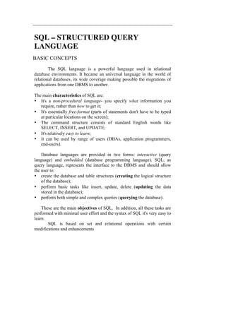
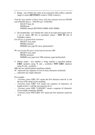
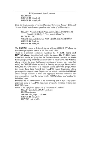
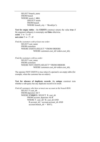
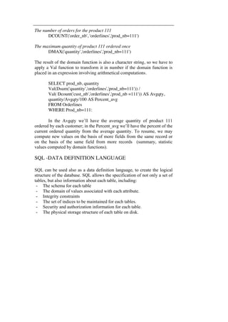
The SELECT statement has the following general form:
SELECT [DISTINCT | ALL] {*| [columnExprn [AS newName]] [,...] }
FROM TableName [alias] [, ...]
[WHERE condition]
[GROUP BY columnList]
[HAVING condition]
[ORDER BY columnList];
where:
- columnExprn represents a column name or an expression
- newName is a name you can give the column as a display heading
- TableName is the name of an existing database table or view that you
have access to
- alias is an optional abbreviation for TableName
Every SQL statement ends with a semicolon (;) to mark the end of the
statement.
The sequence of processing in a SQL statement is:
FROM - Specifies table(s) to be used.
WHERE - Filters rows.
GROUP BY - Forms groups of rows with same column value.
HAVING - Filters groups subject to some condition.
SELECT - Specifies which columns are to appear in output.
ORDER BY - Specifies the order of the output.
- The order of the clauses in the SQL statement cannot be changed.
- Only SELECT and FROM are mandatory; the remainder are optional.
- Every SELECT statement produces a query result table consisting of
one or more columns and zero or more rows.
SQL statements
Examples used in order to explain each SQL statement are based on data
stored in two databases:

The order database for products (orders database):
CUSTOMERS(Cust_nb, Cust_name, Cust_city, Cust_type,Balance)
ORDERS (Order_nb, Order_date, Cust_nb)
ORDERLINES (Order_nb, Prod_nb, Quantity)
PRODUCTS (Prod_nb, Description, MU, Price, Status, Supply_date)
The banking enterprise database (banking database):
BRANCH(branch_nb,branch_name,branch_city,assets)
ACCOUNT(account_nb,branch_nb,balance)
DEPOSITOR(cust_nb,account_nb)
CUSTOMER(cust_nb,cust_name,cust_city)
BORROWER(cust_nb,loan_nb)
LOAN(loan_nb,branch_nb,amount)
The SELECT clause list the attributes desired in the result of a query. It
corresponds to the projection operation of the relational algebra
Find the names of all branches in the loan table
SELECT branch_name
FROM loan
In the “pure” relational algebra syntax, the query would be:
Πbranch_nb(loan)
SQL allows duplicates in tables as well as in query results. To force the
elimination of duplicates, insert the keyword DISTINCT after SELECT.
Find the names of all branches in the loan table, and remove duplicates
SELECT DISTINCT branch-name
FROM loan
The keyword ALL specifies that duplicates not be removed.
SELECT ALL branch_nb
FROM loan
An asterisk in the select clause denotes “all attributes”
SELECT *
FROM loan
The SQL Language offers a large variety of field oriented data processing
by allowing expressions to be inserted in the list of fields of the SELECT
clause. In these expressions we may use any combinations of arithmetical
operators applied to numeric fields (+,-,*,/,^), string operators applied to
character fields (concatenation operator &) and functions.

The query:
SELECT loan_nb, branch_nb, amount *100
FROM loan
would return a table which is the same as the loan table, except that the
attribute amount is multiplied by.
Using the keyword AS we can give a new name either to an existing field,
either to a new (calculated field in the output table).
Suppose we have a table
SALES(Sale_id,Sale_date,Prod_nb,Descript,Qty,Price_unit) and we want
to find out the value of each sale:
SELECT Prod_nb, Descript, Qty, Price_unit AS Price_Per_Unit,
Qty * Price_unit AS Prod_Value
FROM SALES ;
The WHERE clause specifies conditions that the result must satisfy (the
condition has to be met by each record to be selected) and it corresponds
to the selection operator of the relational algebra. The search condition
that specifies the rows to be retrieved is going to have a logical value (true
/ false). The five basic search conditions are:
1. Comparison - compare the value of one expression to the value of
another expression. The comparison operators are: =, >, <., >=, <=,
<>. Comparison results can be combined using the logical connectives
and, or, and not and can be applied to results of arithmetic
expressions.
Find all loan number for loans made at the Perryridge branch with loan
amounts greater than $1000.
SELECT loan_number
FROM loan
WHERE branch_name = ‘Perryridge’ AND amount > 1000;
From table customers in orders database we want to list all new
customers that live in London
SELECT cust_name
FROM customers
WHERE cust_type='new' AND cust_city='LONDON';

2. Range - test whether the value of an expression falls within a specific
range of values (BETWEEN <value1> AND <value2>)
Find the loan number of those loans with loan amounts between $90,000
and $100,000 (that is, >$90,000 and <$100,000)
SELECT loan_nb
FROM loan
WHERE amount BETWEEN 90000 AND 100000;
3. Set membership - test whether the value of an expression equals one of
a set of values: IN (list of permitted values) ; NOT IN (list of
forbidden values)
List all new or preferential customers:
SELECT cust_name
FROM customers
WHERE cust_type IN ('new','preferential');
We can rewrite this query using logical operator OR:
SELECT cust_name
FROM customers
WHERE cust_type='new' OR customer_type='preferential';
4. Pattern match - test whether a string matches a specified pattern:
LIKE <patterns using % and _ symbols>; NOT LIKE <patterns
using % and _ symbols>.
SQL has two special pattern-matching symbols:
% - represents any sequence of zero or more characters (wildcard)
_ - represents any single character
For example:
- Customer_name LIKE 'A%' means the first character must be A, but
the rest of the string can be anything;
- Customer_name LIKE '%A' means any sequence of characters, of
length at least 1, with the last character an A;
- Customer_name LIKE '%ADAM%" means a sequence of characters
of any length containing ADAM;
- Customer_name NOT LIKE 'A%' means the first character cannot be
an A.

Find all customers with name Adam:
SELECT *
FROM customers
WHERE cust_name LIKE 'Adam%';
In some DBMS, such as Microsoft ACCESS, the wildcard characters %
and _ are replaced by * and ?.
5. Null - test whether a column has a null value.
If we want to obtain information about products for which we don't have
established a supply_date (database orders), we can try:
WHERE (supply_date=' ' OR supply_date=0)
But neither of these conditions would work. A null supply_date is
considered to have an unknown value, so we cannot test whether it is
equal or not equal to another value. The result of a query with such a
condition will be an empty table. Instead, we have to test for null
explicitly:
SELECT prod_nb,description
FROM products
WHERE supply_date IS NULL;
The negated version (IS NOT NULL) can be used to test for values that
are not null.
The FROM clause lists the relations involved in the query. It corresponds
to the Cartesian product operation of the relational algebra. In fact, each
query based on more than one table with no WHERE clause is a cartesian
product.
Find the Cartesian product borrower x loan
SELECT* *
FROM borrower, loan
Find the name, loan number and loan amount of all customers
SELECT customer_nb, borrower.loan_nb, amount
FROM borrower, loan
The clause ORDER BY presents the fields whose values will be arranged
in the desired order; if there are more sorting fields, then they are
considered from left to right. The ORDER BY clause must always be the
last clause of the SELECT statement.

List the records in PRODUCTS table in ascending order of description
and for products with the same description in descinding order of prices:
SELECT prod_nb, description, price
FROM products
ORDER BY Description/ASC, Price_unit/DESC ;
List the records in customer table in ascending order of customer name
and balance:
SELECT cust_name, balance
FROM customers
ORDER BY cust_name/ASC, balance/ASC;
Aggregate functions
SUM – returns the sum of the values in a specified column
AVG – returns the average of the values in a specified column
MAX – returns the maximum value in a specified column
MIN – returns the minimum value in a specified column
COUNT – returns the number of values in a specified column
- These functions operate on a single column of a table and returns a
single value. COUNT, MIN, and MAX apply to numeric and non-numeric
fields, but SUM and AVG only for numeric fields.
- Apart from COUNT(*) - a special use of COUNT, which counts all
the rows of a table, including nulls and duplicate values - each
function eliminates nulls first and operates only on remaining non-null
values.
- In order to eliminate duplicates before the function is applied, we use
the keyword DISTINCT before the column name in the function.
Total loan amount
SELECT SUM(amount)
FROM loan;
List the total number of customers with a balance >10000 and the sum of
their balance:
SELECT COUNT(cust_id) AS tcust, SUM(balance) AS totalbalance
FROM customers
WHERE balance>10000;

We apply the count function to count the number of rows satisfying the
WHERE clause and we apply the SUM function to add together the
balances in these rows.
List the minimum, maximum and average values of customer's balance:
SELECT MIN(balance) AS minbal, MAX(balance) AS maxbal,
AVG(balance) AS avgbal
FROM customers;
The clause GROUP BY is used to group records with the same value in
the specified fields.
• A query that includes the GROUP BY clause is called a grouped
query, because it groups the data from the SELECT table and produces
a single summary row for each group. The columns named in the
GROUP BY clause are called the grouping columns.
• Grouping records does not means that the records will be displayed in
groups but for each group only a single record will be presented, a
summary record containing only summarized values of non grouping
fields.
• If the clause GROUP BY is present in the SQL sentence, in the list of
fields and expression of the SELECT clause we may have only
grouping fields names and domain functions applied to one field from
all the records. All field names in the SELECT list must appear in the
GROUP BY clause unless the name is used only in an aggregate
function. But there may be field names in the GROUP BY clause that
do not appear in the SELECT list.
• When the WHERE clause is used with GROUP BY, the WHERE
clause is applied first, then groups are formed from the remaining rows
that satisfy the search condition.
Find the number of customers in London on types:
SELECT cust_type, COUNT(cust_nb)
FROM customers
WHERE cust_city='LONDON'
GROUP BY cust_type;
Find the number of loans for each branch and their total amount:
SELECT branch_nb, COUNT(loan_nb) AS nb_of_loans,

SUM(amount) AS total_amount
FROM loan
GROUP BY branch_nb
ORDER BY branch_nb;
Find the total quantity of each sold product between 1 January 2004 and
31 march 2004 and the corresponding total value of sold products.
SELECT Prod_nb, FIRST(Price_unit) AS Price, SUM(Qty) AS
TotalQ, SUM(Qty * Price_unit) AS TotalVal
FROM SALES
WHERE Sale_date Between #01/01/2004# And #03/31/2004#
GROUP BY Prod_nb
ORDER BY Prod_nb;
The HAVING clause is designed for use with the GROUP BY clause to
restrict the groups that appear in the final result table.
There is a common confusion regarding the WHERE clause and
HAVING clause, since they both restrict the query. The WHERE clause
filters individual rows going into the final result table, whereas HAVING
filters groups going into the final result table. In other words, the WHERE
clause restricts the rows that become members of group - only rows that
satisfy the WHERE clause are used in forming the groups. On the other
hand, the HAVING clause is a selection clause applied to groups. Once
the groups have been formed, the HAVING clause determines which
groups produce output rows. In practice, the search condition in HAVING
clause always includes at least one aggregate function; otherwise the
search condition could be moved to the WHERE clause and applied to
individual rows.
However, the HAVING clause is not a necessary part of SQL - any query
expressed using a HAVING clause can always be rewritten without the
HAVING clause.
Which is the significant type (>10) of customers in London?
SELECT cust_type, COUNT(cust_nb)
FROM customers
WHERE cust_city='LONDON'
GROUP BY cust_type
HAVING cust_nb>10;

Find the number of loans for each branch and their total amount for those
branches in which the loan amount is > 1000000
SELECT branch_nb, COUNT(loan_nb) AS nb_of_loans,
SUM(amount) AS total_amount
FROM loan
GROUP BY branch_nb
ORDER BY branch_nb
HAVING total_amount > 1000000;
Find the total quantity of each sold product between 1 January 2004 and
31 march 2004 and the corresponding total value of sold products but
only for significant sales (meaning sales with Totalval >= 9000000 )
SELECT Prod_nb, FIRST(Price_unit) AS Price, SUM(Qty) AS
TotalQ, SUM(Qty * Price_unit) AS TotalVal
FROM SALES
GROUP BY Prod_nb
ORDER BY Prod_nb,
HAVING TotalVal>=9000000;
An aggregate function can be used only in the SELECT list and in
the HAVING clause. If the SELECT list includes an aggregate function
and no GROUP BY clause is being used to group data together, then no
item in the SELECT list can include any reference to a column unless that
column is the argument to an aggregate function.
For example, the query:
SELECT cust_nb, SUM(balance)
FROM customers;
is illegal, because there is no GROUP BY clause and the field CUST_NB
in the SELECT list is used outside an aggregate function
The INTO clause is used to express the name of a new table where the
result of the query will be permanently stored.
SELECT cust_nb, cust_name, cust_city, balance
FROM customers
WHERE cust_type='new'
INTO newcustomers;

Unless this clause is specified, the result will be displayed to the
user and then lost. The set of records produced by a SQL SELECT
sentence looks and acts like a virtual table, a temporary one. The volatility
is the price for the dynamic aspect of the virtual table, it presents every
time is activated an up to date version of data. If we store a virtual set in a
table, the dynamic aspect is lost. We must recreate the table every time we
need an updated version of data.
In almost all the examples we have considered so far (except those
with FROM clause) we supposed that the result table is based on data
coming from a single table. In many cases, this is no sufficient. In order to
obtain information from several tables, the choice is between using a
subquery and using a join. The SQL join operation combines information
from two tables by forming pairs of related rows from the two tables. The
row pairs that make up the joined table are those where the matching
columns in each of the two tables have the same value.
To perform a join we can
• include more than one table in the FROM clause, using a comma as a
separator and specify the join condition(s) in the WHERE clause, on
the basis of the relational formula:
T1 T2 = σ join predicate ( T1 X T2)
• use the INNER JOIN, LEFT JOIN, RIGHT JOIN, FULL OUTER
JOIN statements in the FROM clause (if the DBMS implements the
join relational operator).
Let's consider the following datasets for examples:
Table LOAN
WHERE FROM
loan_nb branch_nb amount
L1 B10 10000
L3 B20 15000
L2 B40 20000

Table BORROWER
cust_nb loan_nb
C1 L1
C2 L3
C3 L5
INNER JOIN :
List all the loans and their borrowers
SELECT loan.loan_nb,branch_nb,amount,cust_nb
FROM loan,borrower
WHERE loan.loan_nb=borrower.loan_nb;
Or
FROM loan INNER JOIN borrower ON
loan.loan_nb=borrower.loan_nb
Table Loans Borrowers
loan_nb branch_nb amount cust_nb
L1 B10 10000 C1
L3 B20 15000 C2
OUTER JOIN
• LEFT OUTER JOIN - all loans, even they are not
FROM loan LEFT JOIN borrower ON
loan.loan_nb=borrower.loan_nb
The result table Loan Borrower
L1 B10 10000 C1
L3 B20 15000 C2
L2 B40 20000 null

• RIGHT OUTER JOIN -all borrowers, even if they don't have a loan
SELECT borrower.loan_nb,branch_nb,amount,cust_nb
FROM loan RIGHT JOIN borrower ON
loan.loan_nb=borrower.loan_nb;
L1 B10 10000 C1
L3 B20 15000 C2
L5 null null C3
• FULL OUTER JOIN - all loans and all borrowers
SELECT loan.loan_nb, branch_nb,amount,cust_nb
FROM loan FULL OUTER JOIN borrower ON
loan.loan_nb=borrower.loan_nb;
L1 B10 10000 C1
L3 B20 15000 C2
L2 B40 20000 null
L5 null null C3
Find all customers who have either an account or a loan (but not both) at
the bank:
SELECT cust_nb
FROM depositor FULL OUTER JOIN borrower
ON depositor.cust_nb=borrower.cust_nb
WHERE account_number IS null or loan_nb IS null;
List of products ordered by customer '1111':
SELECT description
FROM products,orderedproducts,orders,customers
WHERE customers.cust_nb=orders.cust_nb
AND orders.order_nb=orderlines.order_nb
AND orderlines.prod_nb=products.prod_nb

AND customers.cust_nb='1111';
Or
SELECT description
FROM products INNER JOIN ((customers INNER JOIN orders
ON customers.cust_nb = orders.custnb) INNER JOIN orderlines
ON orders.order_nb = orderlines.order_nb) ON products.prod_nb
= orderlines.prod_nb
WHERE customers.cust_nb='1111';
Alphabetical list of products ordered today:
SELECT description
FROM products,orderlines,orders
WHERE products.prod_nb=orderlines.prod_nb
AND orderlines.order_nb= orders.order_nb
AND orders.order_date=Date()
ORDER BY description;
Or
SELECT description
FROM orders INNER JOIN (products INNER JOIN orderline ON
products.prod_nb=orderlines.prod_nb) ON
orders.order_nb = orderlines.order_nb
WHERE orders.order_date=Date()
ORDER BY description;
Subqueries
Some SQL queries are so complex that they won't fit into the form
of a single SELECT statement. The SQL sentences cannot be chained to
be executed one after the other (algorithm like) but they can be nested
(imbricate) as subsequent SELECT sentences in WHERE and HAVING
clauses. The results of this inner SELECT statement (subselect) are used
in the outer statement to help determine the contents of the final result.
SQL provides a mechanism for the nesting of subqueries. A
subquery is a SELECT-FROM-WHERE expression that is nested within

another query. We can think of the subquery as producing a temporary
table with results that can be accessed and used by the outer statement. A
subquery can be used immediately following an operator(<,>,=,>=,<=,<>)
in a WHERE clause or a HAVING clause. The subquery itself is always
enclosed in parentheses.
The imbricate SELECT sentence could be inserted as a source for a list of
permitted or forbidden values used with IN or NOT IN operators.
Find all customers who have both an account and a loan at the bank:
SELECT DISTINCT cust_nb
FROM borrower
WHERE cust_nb IN (SELECT cust_nb FROM depositor);
Find all customers who have a loan at the bank but do not have an
account at the bank:
SELECT DISTINCT cust_nb
FROM borrower
WHERE cust_nb NOT IN (SELECT cust_nb FROM depositor)
The subsequent SQL could select only one field (except for those that use
the keyword EXISTS). We can use the string operator & to concatenate
more fields in an expression.
Find the orders not invoiced the same day they were taken:
SELECT Cust_nb, Prod_nb, Ord_date,Qty
FROM ORDERS
WHERE Prod_nb & Cust_nb & Ord_date NOT IN
(SELECT Prod_nb & Cust_nb & Invoice_date
FROM INVOICES);
Find unsatisfied orders (no invoices for the Cust_nb specifying the total
value of that Cust_nb’s order):
SELECT Cust_nb, SUM (Qty * Price_unit) AS TotalVal
FROM ORDERS, PRODUCTS
GROUP BY Cust_nb
WHERE ORDERS. Prod_nb = PRODUCTS.Prod_nb

HAVING Cust_nb & TotalVal NOT IN
( SELECT Cust_nb & TotalVal
FROM INVOICES);
Subqueries are used also with aggregate function. An aggregate function
can be used only in the SELECT list and in the HAVING clause. So, it
would be wrong to write 'WHERE price > AVG(price)'. Instead, we use a
subquery to find the average price and then use the outer SELECT
statement to find those products with prices greater than the average price:
SELECT prod_nb, description
FROM products
WHERE price > (SELECT AVG(price)
FROM products);
Note that the ORDER BY clause may not be used in a subquery (although
it may be used in the outermost SELECT statement).
A common use of subqueries is to perform tests for set membership, set
comparisons, and set cardinality. The operators and keywords that we can
use in a nested SELECT statement are: IN, NOT, ALL, EXISTS, EXISTS,
UNIQUE, CONTAINS, UNION, INTERSECTION, SOME,ANY
Set comparison - ANY, ALL, SOME
SOME - all records that satisfy the comparison with some
resulting records of the subquery (note that (= some) = in and (≠ some)
<>not in )
Find all branches that have greater assets than some branch located in
Brooklyn.
SELECT branch_name
FROM branch
WHERE assets > SOME
(SELECT assets
FROM branch WHERE branch_city = ‘Brooklyn’)
ALL - all records that satisfy the comparison with all resulting
records of the subquery ( note that (≠ all) = not in and (= all) <> in)
Find the names of all branches that have greater assets than all branches
located in Brooklyn:

SELECT branch_name
FROM branch
WHERE assets > ALL
(SELECT assets
FROM branch
WHERE branch_city = ‘Brooklyn’);
Test for empty tables - the EXISTS construct returns the value true if
the argument subquery is nonempty and false otherwise.
exists T ⇔ T ≠ Ø
not exists T ⇔ T = Ø
Find the customers with at least one order:
SELECT cust_name
FROM customers
WHERE EXISTS (SELECT * FROM ORDERS
WHERE customers.cust_nb=orders.cust_nb);
Find the customers with no order:
SELECT cust_name
FROM customers
WHERE NOT EXISTS (SELECT * FROM ORDERS
WHERE customers.cust_nb=orders.cust_nb);
The operator NOT EXISTS is true when it's operand is an empty table (for
example, when the customer has no orders).
Test for absence of duplicate records: the unique construct tests
whether a sub-query has any duplicate record in its result.
Find all customers who have at most one account at the branch B10:
SELECT T.cust_nb
FROM depositor AS T
WHERE UNIQUE ( SELECT R. cust_nb
FROM account, depositor AS R
WHERE T. cust_nb= R. cust_nb AND
R.account_nb = account.account_nb AND
account.branch_nb = ‘B10’);

Find all customers who have at least two accounts at the branch B10:
SELECT T.cust_nb
FROM depositor AS T
WHERE NOT UNIQUE ( SELECT R. cust_nb
FROM account, depositor AS R
WHERE T. cust_nb= R. cust_nb AND
R.account_nb = account.account_nb AND
account.branch_nb = ‘B10’);
Set operations
SQL can perform union, intersection and difference operations. The set
operations union, intersect, and except operate on relations and
correspond to the relational algebra operations ∪, ∩, −. These operations
automatically eliminates duplicates; to retain all duplicates use the
corresponding multiset versions union all, intersect all and except all.
Suppose a record occurs m times in T1and n times in T2, then, it
occurs:
- m + n times in T1 union all T2
- min(m,n) times in T1 intersect all T2
- max(0, m – n) times in T1 except all T2
The UNION clause is used to merge (concatenate) the result of two select
sentences. The syntax of the second select is independent except the list of
fields and expressions that must be the same (the union is performed on
tables with the same structure).
Find all customers (source tables are customers2003 and customers2004
and have the same logical structure):
(SELECT * FROM customers2003)
UNION
(SELECT * FROM customers2004);
Find all customers who have a loan, an account, or both:
(SELECT cust_nb FROM depositor)
UNION
(SELECT cust_nb FROM borrower);

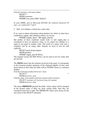
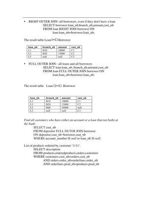
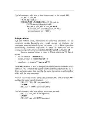
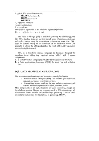
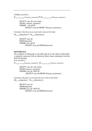
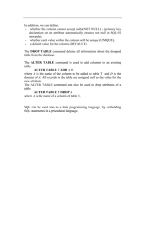
The INTERSECT clause will return records belonging to both tables.
Find the faithful customers (customers2003 ∩ customers2004):
INTERSECT
(SELECT *FROM customers2004);
Find all customers who have both a loan and an account:
INTERSECT
The EXCEPT clause is used for difference and will return those records
belonging to the first table and not to the second one:
Lost customers (customers2003 - customers2004):
EXCEPT
(SELECT *FROM customers2004);
Find all customers who have an account but no loan:
EXCEPT
We can implement set relational operators also by using nested queries, as
we'll discuss later in this chapter.
Modification of the database
SQL is a complete data manipulation language that can be used for
modifying the data in the database as well as querying the database. The
requests for updating data in the database are expressed with the following
statements:
- INSERT adds new rows of data (records) in a table.
- UPDATE modifies existing data in a table.
- DELETE removes rows of data from a table.
The general format of the INSERT statement is
INSERT INTO tablename[(list of fields)]
VALUES (data value list);

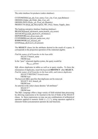
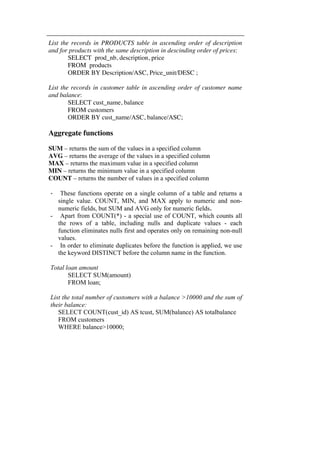
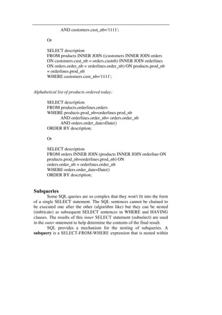
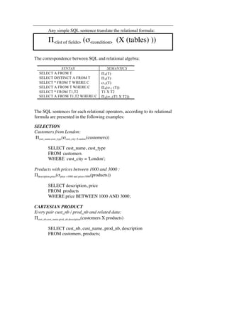
where tablename is the name of a base table and list of fields represents a
list of one or more field's names separated by commas. The list of fields is
optional; if omitted, SQL assumes all columns of the table. The data
value list must match the list of fields as follows:
- the number of items in each list must be the same;
- there must be a direct correspondence in the position of items in the
two lists;
- the data type of each item in data value list must be compatible with
the data type of the corresponding field in list of fields.
Add a new tuple to account
INSERT INTO account
VALUES (‘A100’, ‘B7’,1500)
or equivalently
INSERT INTO account (branch_nb, balance, account_nb)
VALUES (‘B7’, 1500, ‘A100’);
The list of values associated with table fields can be produced by an
imbricate select sentence. The SELECT FROM WHERE statement is fully
evaluated before any of its results are inserted into the table.
INSERT INTO tablename[(list of fields)]
SELECT <…. >
FROM <….>
[WHERE <…> ];
The pairs field name values must be done in the subsequent select like in
the following examples:
In the SALES file we add daily the sales made by the retail department
(stored in RETAIL table). For the Descript field where we do not have
values we’ll add a null value to match the SALES table list of fields:
INSERT INTO SALES (Prod_nb, Descript, Qty, Price_unit,
Prod_Value)
SELECT Prod_id AS Prod_nb, null AS Descript, Q AS Qty,
Price AS Price_unit , Qty * Price_unit AS Prod_Value
FROM RETAIL
WHERE Retail_date=Date();

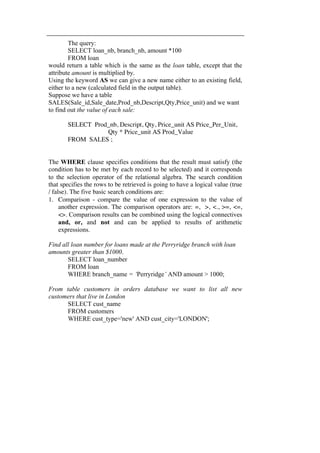
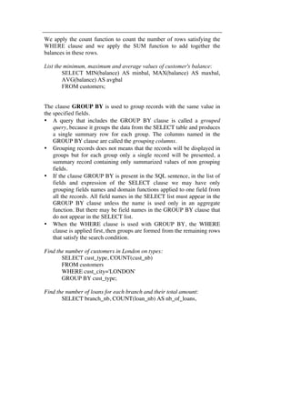
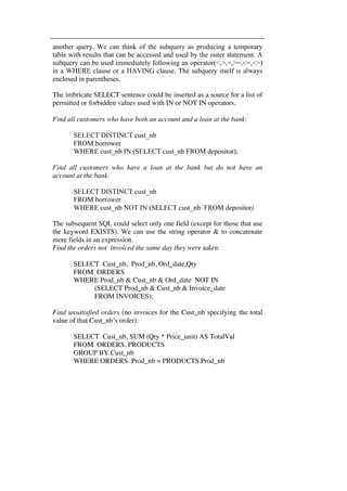
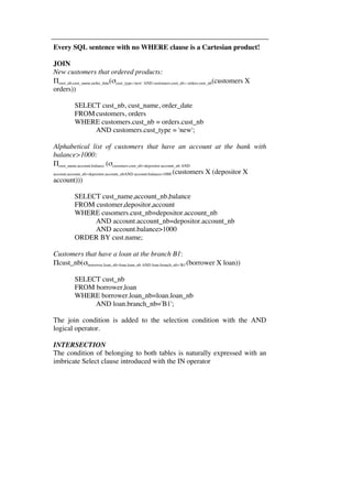
Provide as a gift for all loan customers of the branch B1, a $200 savings
account. Let the loan number serve as the account number for the new
savings account
INSERT INTO account
SELECT loan_nb, branch_nb, 200
FROM loan
WHERE branch_nb = ‘B1’;
INSERT INTO depositor
SELECT cust_nb, loan_nb
FROM loan, borrower
WHERE branch_nb = ‘B1’
and loan.account_nb = borrower.account_nb;
The format of the UPDATE statement is:
UPDATE tablenane
SET field1=datavalue1/expression1
[,field2=datavalue2/expression2…..]
[WHERE conditions to be met by each record to be updated];
Increase all accounts with balances over $50,000 by 6%, all other
accounts receive 5%.
Write two update statements:
UPDATE account
SET balance = balance ∗ 1.06
WHERE balance > 50000;
UPDATE account
SET balance = balance ∗ 1.05
WHERE balance <= 50000;
We can answer to that request writing a single query if we use the CASE
statement :
UPDATE account
SET balance = CASE
WHEN balance <= 50000 THEN balance *1.05

ELSE balance * 1.06
END;
The format of the DELETE statement:
DELETE FROM tablename
[WHERE < condition to be met by each record to be deleted>];
Records that will meet the condition (or all records, if we don't specify any
condition) will be permanently deleted.
Delete all the records referring to retail sales made before today :
DELETE FROM RETAIL
WHERE Retail_date<Date()
Delete the record of all accounts with balances below the average at the
bank.
DELETE FROM account
WHERE balance < (SELECT AVG (balance)
FROM account);
Insertion, deletion and update are permanent data processing; they alter
data in the database and cannot be undone. For this reason, they must be
performed carefully and only once. If by accident they are repeated, data is
irreversibly altered.
SQL and relational algebra
The SQL language is build on a small set of minimal relational operators
provided by the Data Base Management System: Selection, Projection and
Cartesian Product
SELECT < list of fields > Projection
FROM < list of tables > Cartesian product
WHERE < list of conditions > Selection

Any simple SQL sentence translate the relational formula:
Π<list of fields> (σ<condition> (X (tables) ))
The correspondence between SQL and relational algebra:
SYNTAX SEMANTICS
SELECT A FROM T ΠA(T)
SELECT DISTINCT A FROM T ΠA(T)
SELECT * FROM T WHERE C σ C(T)
SELECT A FROM T WHERE C ΠA(σ C (T))
SELECT * FROM T1,T2 T1 X T2
SELECT A FROM T1,T2 WHERE C ΠA(σ C(T1 X T2))
The SQL sentences for each relational operators, according to its relational
formula are presented in the following examples:
SELECTION
Customers from London:
Πcust_name,cust_type(σcust_city='London'(customers))
SELECT cust_name, cust_type
FROM customers
WHERE cust_city = 'London';
Products with prices between 1000 and 3000 :
Πdescription,price(σprice >1000 and price<3000(products))
SELECT description, price
FROM products
WHERE price BETWEEN 1000 AND 3000;
CARTESIAN PRODUCT
Every pair cust_nb / prod_nb and related data:
Πcust_nb,cust_name,prod_nb,description(customers X products)
SELECT cust_nb, cust_name, prod_nb, description
FROM customers, products;

Every SQL sentence with no WHERE clause is a Cartesian product!
JOIN
New customers that ordered products:
Πcust_nb,cust_name,order_date(σcust_type='new' AND customers.cust_nb= orders.cust_nb(customers X
orders))
SELECT cust_nb, cust_name, order_date
FROM customers, orders
WHERE customers.cust_nb = orders.cust_nb
AND customers.cust_type = 'new';
Alphabetical list of customers that have an account at the bank with
balance>1000:
Πcust_name,account,balance (σcusomers.cust_nb=depositor.account_nb AND
account.account_nb=depositor.account_nbAND account.balance>1000 (customers X (depositor X
account)))
SELECT cust_name,account_nb,balance
FROM customer,depositor,account
WHERE cusomers.cust_nb=depositor.account_nb
AND account.account_nb=depositor.account_nb
AND account.balance>1000
ORDER BY cust.name;
Customers that have a loan at the branch B1:
Πcust_nb(σborrower.loan_nb=loan.loan_nb AND loan.branch_nb='B1'(borrower X loan))
SELECT cust_nb
FROM borrower,loan
WHERE borrower.loan_nb=loan.loan_nb
AND loan.branch_nb='B1';
The join condition is added to the selection condition with the AND
logical operator.
INTERSECTION
The condition of belonging to both tables is naturally expressed with an
imbricate Select clause introduced with the IN operator

Faithful_customers :
Π cust_nb,cust_name (Lastyear_customers) ∩ Π cust_nb,cust_name (Thisyear_customers )
SELECT cust_nb, cust_name,
FROM Lastyear_customers
WHERE cust-nb IN
(SELECT cust_nb FROM Thisyear_customers);
Customers that have an account and a loan at the bank:
(Πcust_nb(depositor) ∩ Πcust_nb(borrower)):
SELECT cust_nb
FROM depositor
WHERE cust_nb IN
DIFFERENCE
The condition of belonging to one table and not to the other to both tables
is naturally expressed with an imbricate Select clause introduced with the
NOT IN operator
Lost customers:
Π cust_nb, cust_name(Lastyear_customers) - Π cust_nb, cust_name (Thisyear_customers)
SELECT cust_nb, cust_name,
FROM Lastyear_customers
WHERE cust_nb NOT IN
(SELECT cust_nb FROM Thisyear_customers);
Customers that have an account but not a loan at the bank:
(Πcust_nb(depositor) - Πcust_nb(borrower)):
SELECT cust_nb
FROM depositor
WHERE cust_nb NOT IN

UNION
Customers that have an account, a loan or both at the bank:
(Πcust_nb(depositor) U Πcust_nb(borrower))
SELECT cust_nb FROM depositor
UNION
SELECT cust_nb FROM borrower;
Any complex process diagram can be translated easily in SQL sentences,
once the set of relational operators identified, for each we have to write an
SQL sentence with an INTO clause to preserve the result to be used in
other SQL sentence. Chaining SQL sentences in the order required by the
diagram is the user concern. However, many DBMS preserve the SQL
sentence in an ready to use form associated with a name behaving like a
virtual table that can be used as a basis for an other SQL sentence. This
mechanism eliminate the disadvantage of not being able to express an
imbricate SQL sentence in the FROM clause.
Functions
The SQL Language offers a large variety of field oriented data processing
by allowing expressions to be inserted in the list of fields of the SELECT
clause.
In these expressions we may use any combinations of arithmetical
operators applied to numeric fields (+,-,*,/,^), string operators applied to
character fields (concatenation operator &) and functions
- Val(text field) – transform text in number
- Str(numeric field) – transform number in text
- Nz(numeric field) – transform null fields in number fields with zero
value
We may also use functions to choose a value for the new data according to
a condition. This functions enable the user to express very complicated
data processing:
The IIF function with the syntax:
IIF(condition, expression for true, expression for false) AS Newdata

The condition is a logical expression evaluated for every record. If
the condition is met (the logical value is true) then the expression for true
is computed and the value is chosen for the Newdata, if the condition is
not met, then the expression for false is taken into consideration to
produce the value for Newdata. Both the expression for true and for false
might contain another Iif functions, so we can express any algorithm here.
Example:
In Orders database, we want to insert in a table called DISCOUNT data on
discounts for customers, established on the basis of total ordered value by
each customer. Depending on the customer type (New, Preferential,
Regular), the discount percent is calculated after the following scheme:
Cust_type 10000-20000 20000-50000 >50000
New 5% 7% 9%
Preferenti
8% 10% 12%
al
Regular 3% 5% 8%
INSERT INTO discount (Cust_nb,totalvalue,discpercent)
SELECT cust_nb, SUM(price*quantity) AS totalvalue,
Iif(cust_type ='new', Iif (totalvalue < =10000,0,
Iif(totalvalue <20000,0.05,
iif(totalvalue <=50000,0.7,0.9))),
Iif(cust_type='preferential', Iif(totalvalue <=10000,0,
Iif(totalvalue <=20000, 0.08,
iif(totalvalue <=50000,0.1,0.12))),
Iif (cust_type='regular',Iif(totalvalue <=10000,0,
iif(totalvalue <=20000,0.03
iif(totalvalue<=50000,0.05,0.08))))))
AS discpercent
FROM customers, orders, orderlines,products
GROUP BY cust_nb;

Or, if we restrict records in Discount table (we want to insert only those
records regarding customers that ordered significant values - > 10000)
using HAVING clause:
INSERT INTO discount (Cust_nb,totalvalue,discpercent)
SELECT cust_nb, SUM(price*quantity) AS totalvalue,
Iif(cust_type ='new', Iif(totalvalue <20000,0.05,
iif(totalvalue <=50000,0.7,0.9)),
Iif(cust_type='preferential', Iif((totalvalue <=20000, 0.08,
iif(totalvalue <=50000,0.1,0.12)),
Iif (cust_type='regular',Iif(totalvalue <=20000,0.03
iif(totalvalue<=50000,0.05,0.08)))))
AS discpercent
FROM customers, orders, orderlines,products
GROUP BY cust_nb
HAVING totalvalue>10000;
Another functions widely used are domain functions: functions applied
on a set of values extracted from the same field taken from a set of records
from a table. These domain function perform the selection of records from
a specific table (not the ones in the FROM clause) on a given condition
and then summarize a specific field of them (sum, count, min, max). They
are in fact the same summary functions used in Select sentences with the
GROUP BY clause. But there, the domain is the group of records taken
from the tables designated in the FROM clause, while in this approach,
the domain is a selection of records taken from an outer table not specified
in the FROM list, records meeting a condition not included in the
WHERE clause. For instance:
DSUM ('field', 'table ', 'condition')
produces the sum of values stored in the “field” from the records of the
“table” that meet the “condition”. The arguments of the domain functions
are string of characters enclosed in ' '.
The sum of quantities ordered on the product 111
DSUM('quantity', 'orderlines', 'prod_nb=111')

The number of orders for the product 111
DCOUNT('order_nb', 'orderlines','prod_nb=111')
The maximum quantity of product 111 ordered once
DMAX('quantity','orderlines','prod_nb=111')
The result of the domain function is also a character string, so we have to
apply a Val function to transform it in number if the domain function is
placed in an expression involving arithmetical computations.
SELECT prod_nb, quantity
Val(Dsum('quantity','orderlines','prod_nb=111')) /
Val( Dcount('cust_nb','orderlines','prod_nb =111')) AS Avgqty,
quantity/Avgqty/100 AS Percent_avg
FROM Orderlines
WHERE Prod_nb=111:
In the Avgqty we’ll have the average quantity of product 111
ordered by each customer; in the Percent_avg we’ll have the percent of the
current ordered quantity from the average quantity. To resume, we may
compute new values on the basis of more fields from the same record or
on the basis of the same field from more records (summary, statistic
values computed by domain functions).
SQL -DATA DEFINITION LANGUAGE
SQL can be used also as a data definition language, to create the logical
structure of the database. SQL allows the specification of not only a set of
tables, but also information about each table, including:
- The schema for each table
- The domain of values associated with each attribute.
- Integrity constraints
- The set of indices to be maintained for each tables.
- Security and authorization information for each table.
- The physical storage structure of each table on disk.

CREATE TABLE statement:
CREATE TABLE TableName
{(columnName dataType [NOT NULL] [UNIQUE]
[DEFAULT defaultOption][,...]}
[PRIMARY KEY (listOfColumns),]
{[UNIQUE (listOfColumns),] […,]}
{[FOREIGN KEY (listOfFKColumns)
REFERENCES ParentTableName [(listOfCKColumns)],
[ON UPDATE referentialAction]
[ON DELETE referentialAction ]] [,…]}
Example: Create table branch, declare branch_nb as the primary key for
branch and ensure that the values of assets are non-negative.
CREATE TABLE branch
(branch_nb char (4)
branch-name char(15),
branch-city char(30)
assets integer,
PRIMARY KEY (branc_nb),
CHECK (assets >= 0)) ;
The basic format for defining a column of a table
(columnName dataType [NOT NULL] [UNIQUE]
[DEFAULT defaultOption][,...]
where columnname is the name of the column and datatype defines the
type of the column. The most widely used data types are:
- CHARACTER(L) (CHAR) - defines a string of fixed length L.
- CHARACTER VARYING(L) (VARCHAR) - defines a string of
varying length L.
- DECIMAL (precision,[scale]) or NUMERIC(precision,[scale]) -
defines a string with an exact representation: precision specifies the
number of significant digits and scale specifies the number of digits
after the decimal point.
- INTEGER and SMALLINT- define numbers where the representation
of fractions is not required.
- DATE - stores data values in Julian format as a combination of
YEAR (4 digits), MONTH (2 digits), and DAY(2 digits).

In addition, we can define:
- whether the column cannot accept nulls(NOT NULL) - (primary key
declaration on an attribute automatically ensures not null in SQL-92
onwards);
- whether each value within the column will be unique (UNIQUE);
- a default value for the column (DEFAULT).
The DROP TABLE command deletes all information about the dropped
table from the database.
The ALTER TABLE command is used to add columns to an existing
table.
ALTER TABLE T ADD A D
where A is the name of the column to be added to table T and D is the
domain of A. All records in the table are assigned null as the value for the
new attribute.
The ALTER TABLE command can also be used to drop attributes of a
table
ALTER TABLE T DROP A
where A is the name of a column of table T.
SQL can be used also as a data programming language, by embedding
SQL statements in a procedural language.

Sql

Recommended

Recommended

More Related Content

What's hot

What's hot (20)

Similar to Sql

Similar to Sql (20)

More from Diana Diana

More from Diana Diana (20)

Sql