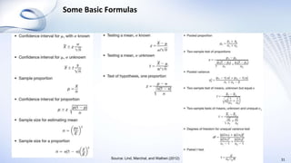
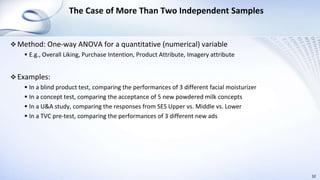
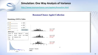
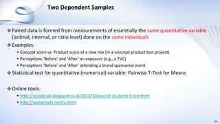
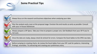
This document provides an overview of data analysis and statistics concepts for a training session. It begins with an agenda outlining topics like descriptive statistics, inferential statistics, and independent vs dependent samples. Descriptive statistics concepts covered include measures of central tendency (mean, median, mode), measures of variability (range, standard deviation), and charts. Inferential statistics discusses estimating population parameters, hypothesis testing, and statistical tests like t-tests, ANOVA, and chi-squared. The document provides examples and online simulation tools. It concludes with some practical tips for data analysis like checking for errors, reviewing findings early, and consulting a statistician on analysis plans.

1. Data Analysis and Statistics
PERPI Training
Hotel Puri Denpasar
March 30, 2017
Version 2
by T.S. Lim
Quantitative Senior Research Director and Partner
Leap Research

2. 2

3. Agenda
3
1 What is Statistics?
2 Types of Variables and Levels of Measurement
3 Descriptive Statistics
4 Inferential Statistics
5 Independent and Dependent Samples

4. References
 Carr, Rodney. Practical Statistics. XLent Works.
http://www.deakin.edu.au/~rodneyc/PracticalStatistics/, 2013
 Gonick, Larry, and Woollcott Smith. The Cartoon Guide to Statistics (New York:
HarperPerennial, 2015), Kindle edition
 Lind, Douglas A., William G. Marchal, and Samuel A. Wathen. Statistical Techniques in
Business & Economics. 15th ed. New York: McGraw-Hill/Irwin, 2012
 Malhotra, Naresh K. Marketing Research: An Applied Orientation. Global Edition, 6th ed.
Upper Saddle River: Pearson Education, 2010
 Rumsey, Deborah. Statistics Essentials For Dummies. Hoboken: Wiley, 2010
4

5. What is Statistics?

6. 6

7. Statistics
 The science of collecting, organizing, presenting,
analyzing, and interpreting data to assist in
making more effective decisions
 2 categories: descriptive statistics and inferential
statistics
 DESCRIPTIVE STATISTICS: Methods of organizing,
summarizing, and presenting data in an
informative way
 E.g., via various charts, tables, infographics
 INFERENTIAL STATISTICS: The methods used to
estimate a property of a population on the basis
of a sample
 E.g., T-Test, Z-Test, ANOVA, Regression Analysis,
Factor Analysis, Cluster Analysis
7Source: Lind, Marchal, and Wathen (2012)

8. Ethics and Statistics
 A guideline can be found in the paper “Statistics and Ethics: Some Advice for Young Statisticians,”
in The American Statistician 57, no. 1 (2003)
 The authors advise us to practice statistics with integrity and honesty, and urge us to “do the right
thing” when collecting, organizing, summarizing, analyzing, and interpreting numerical
information
 The real contribution of statistics to society is a moral one. Financial analysts need to provide
information that truly reflects a company’s performance so as not to mislead individual investors.
 Information regarding product defects that may be harmful to people must be analyzed and
reported with integrity and honesty
 The authors of The American Statistician article further indicate that when we practice statistics,
we need to maintain “an independent and principled point-of-view”
8Source: Lind, Marchal, and Wathen (2012), page 14
In Marketing Research, we change the data values only when it’s clearly justifiable; e.g., data entry or coding
error. We must never change the values just to increase / decrease the mean score.

9. Types of Variables and Levels of Measurement

10. Types of Variables
10Source: Lind, Marchal, and Wathen (2012)

11. Ratio Level
Interval Level
Ordinal Level
Nominal Level
Four Levels of Measurement
11
It has all the characteristics of the interval level, and additionally the 0
point is meaningful and the ratio between two numbers is meaningful
It includes all the characteristics of the ordinal level, and additionally the
difference between values is a constant size
Data are represented by sets of labels or names; they have relative values and
hence they can be ranked or ordered
Observations of a qualitative variable can only be classified and counted
Data can be classified according to levels of measurement. The level of measurement of
the data dictates the calculations that can be done to summarize and present the data. It
will also determine the statistical tests that should be performed.
Source: Lind, Marchal, and Wathen (2012)

12. Four Levels of Measurement
Summary
12
In Marketing Research, we usually assume that variables of non Nominal level to have at least Interval level
Source: Lind, Marchal, and Wathen (2012)

13. Descriptive Statistics

14. Measures of Location
 Measures of location that we discuss are measures of central tendency because they tend
to describe the center of the distribution
 If the entire sample is changed by adding a fixed constant to each observation, then the mean, mode
and median change by the same fixed amount
 Mean: The mean, or average value, is the most commonly used measure of central
tendency
 The measure is used to estimate the unknown population mean when the data have been collected
using an interval or ratio scale
 The data should display some central tendency, with most of the responses distributed around the
mean
 Note: Sample Mean is prone to the presence of outliers (very big or very small numbers) in the data
14Source: Malhotra (2010)

15. Measures of Location (Cont.)
 Mode: The mode is the value that occurs most frequently
 It represents the highest peak of the distribution
 The mode is a good measure of location when the variable is inherently categorical or has otherwise
been grouped into categories
 Median: The median of a sample is the middle value when the data are arranged in
ascending or descending order
 If the number of data points is even, the median is usually estimated as the midpoint between the two
middle values by adding the two middle values and dividing their sum by 2
 The median is the 50th percentile
 The median is an appropriate measure of central tendency for ordinal data
 Note: Sample Median is robust to the presence of outliers in the data. However, the mathematics
involved in dealing with median and ordinal level data in general is difficult.
15

16. The Relative Positions of the Mean, Median, and Mode
16Source: Lind, Marchal, and Wathen (2012)

17. Measures Variability
 The measures of variability, which are calculated on interval or ratio data, include the
range, interquartile range, variance or standard deviation, and coefficient of variation
 Range: The range measures the spread of the data
 It is simply the difference between the largest and smallest values in the sample
 Interquartile Range (IQR): The interquartile range is the difference between the 75th and
25th percentiles
 For a set of data points arranged in order of magnitude, the pth percentile is the value that has p% of
the data points below it and (100 – p)% above it
 If all the data points are multiplied by a constant, the interquartile range is multiplied by the same
constant
17Source: Malhotra (2010)

18. Measures Variability (Cont.)
 Variance: The difference between the mean and an observed value is called the deviation
from the mean. The variance is the mean squared deviation from the mean.
 The variance can never be negative
 When the data points are clustered around the mean, the variance is small. When the data points are
scattered, the variance is large.
 If all the data values are multiplied by a constant, the variance is multiplied by the square of the
constant
 Standard Deviation: The standard deviation is the square root of the variance
 Thus, the standard deviation is expressed in the same units as the data, rather than in squared units
(like in the variance)
 Coefficient of Variation: The coefficient of variation is the ratio of the standard deviation
to the mean expressed as a percentage, and it is a unitless measure of relative variability
18

19. 19
FunnelRadar Combo
Column Line Bar
Example of Charts (1)

20. 20
Waterfall Histogram Pareto
Box & Whisker Treemap Sunburst
Example of Charts (2)

21. Inferential Statistics

22. Estimating a Population Parameter: Making Your Best
Guesstimate
 We want to estimate a population parameter (a single number that describes a
population) by using statistics (numbers that describe a sample of data)
 Examples:
 Estimating Overall Liking score of a new product
 Estimating Customer Satisfaction Index
 Estimating the average units purchased per purchase occasion
 Estimating % agreement to a statement
 Types of estimates:
 Point Estimate  one single number only
 Interval Estimate  an interval containing a range of numbers (called Confidence Interval)
22

23. Simulation: One Proportion Inference
23
http://www.rossmanchance.com/applets/OneProp/OneProp.htm
0.000
0.005
0.010
0.015
0.020
0.025
0.030
0.035
0.040
0 0.1 0.2 0.3 0.4 0.5 0.6 0.7 0.8 0.9 1
StandardError Proportion
The highest Standard
Error for Proportion is
achieved at p = 0.5
When the Proportions are
small or big, the Standard
Errors are small

24. Simulation: Confidence Intervals for Means
24
http://www.rossmanchance.com/applets/ConfSim.html

25. A General Procedure for Hypothesis Testing
25
HYPOTHESIS TESTING
A procedure based on sample evidence
and probability theory to determine
whether the hypothesis is a reasonable
statement
Examples:
 The heavy and light users of a brand differ
in terms of psychographics characteristics
 One hotel has a more upscale image than
its close competitor
 Concept A is rated higher than Concept B on
Overall Liking
Source: Malhotra (2010)

26. Type I and Type II Errors in Hypothesis Testing
26
Alpha (α) is the probability of making a Type I error 
We want α to be as low as possible!
Beta (β) is the probability of making a Type II error.
The power of a test is the probability (1 – β) of rejecting
the null hypothesis when it is indeed false and hence
should be rejected  We want power to be as high as
possible!
Unfortunately, α and β are interrelated. So, it’s necessary
to balance the two types of errors.
The level of α along with the sample size will determine
the level of β for a particular research design.
In practice, we usually set α at 1%, 5%, or 10%.
The risk of both α and β can be controlled by
increasing the sample size.
For a given level of α, increasing the sample size
will decrease β, and hence increasing the power
of the test (1 – β).
Think of sample size as a magnifying glass.
Sources: Lind, Marchal, and Wathen (2012). Malhotra (2010).

27. Hypothesis Tests Related to Differences
27
Interval or Ratio Level Nominal or Ordinal Level
Source: Malhotra (2010)

28. Independent and Dependent Samples

29. Two Independent Samples: Evaluating the Difference between
Two Mean Scores
 The data come from 2 unrelated samples, drawn randomly from different populations
 The 2 samples are not experimentally related. The measurement of one sample has no
effect on the values of the second sample.
 Note: In a monadic design, the samples are independent
 Examples
 Comparing the Purchase Intent mean scores of Concept X vs. Concept Y
 Comparing the responses of Females vs. Males
 Comparing the reaction towards TVC A vs. TVC B
 Online tools:
 http://www.evanmiller.org/ab-testing/t-test.html
 http://www.quantitativeskills.com/sisa/statistics/t-test.htm
29

30.  The data also come from 2 unrelated samples, but we focus on evaluating the
proportions
 Examples: comparing Top Box, Top 2 Boxes, Bottom Box, Bottom 2 Boxes, Brand
Association
 Caution: declaring 2 proportions as statistically significantly different when the actual
difference is small
 An online tool: http://www.evanmiller.org/ab-testing/chi-squared.html
30
Two Independent Samples: Evaluating the Difference between
Two Proportions
T2B Differences:
Proto 1 (a) – Proto 2 (b) = 5%
Proto 1 (a) – Proto 4 (d) = 4%
Product Attribute Proto 1 Proto 2 Proto 3 Proto 4 Competitor
(a) (b) (c) (d) (e)
Respondents Base 247 242 241 246 244
Cleans hair very well T2B 93% 88% 92% 89% 92%
bd
Means 4.43 4.45 4.47 4.51 4.46

31. Some Basic Formulas
31Source: Lind, Marchal, and Wathen (2012)

32. The Case of More Than Two Independent Samples
 Method: One-way ANOVA for a quantitative (numerical) variable
 E.g., Overall Liking, Purchase Intention, Product Attribute, Imagery attribute
 Examples:
 In a blind product test, comparing the performances of 3 different facial moisturizer
 In a concept test, comparing the acceptance of 5 new powdered milk concepts
 In a U&A study, comparing the responses from SES Upper vs. Middle vs. Lower
 In a TVC pre-test, comparing the performances of 3 different new ads
32

33. Simulation: One Way Analysis of Variance
33
http://www.rossmanchance.com/applets/AnovaSim.html

34. Two Dependent Samples
 Paired data is formed from measurements of essentially the same quantitative variable
(ordinal, internal, or ratio level) done on the same individuals
 Examples:
 Concept score vs. Product score of a new mix (in a concept-product test project)
 Perceptions ‘Before’ and ‘After’ an exposure (e.g., a TVC)
 Perceptions ‘Before’ and ‘After’ attending a brand sponsored event
 Statistical test for quantitative (numerical) variable: Pairwise T-Test for Means
 Online tools:
 http://scistatcalc.blogspot.co.id/2013/10/paired-students-t-test.html
 http://vassarstats.net/tu.html
34

35. The Case of More Than Two Dependent Samples
35
7.53
7.07
7.03
6.37
7.52 7.79
4
5
6
7
8
9
Week 1 Week 2 Week 3
Usage(grams)
Females Males
Total Usage Females : 21.63 grs / person
Total Usage Males : 21.68 grs / person
(***)
(***) vs.
Week 1
(xxx)
(xxx) (xxx) vs.
Week 1
Deodorant Usage in 3-Week Period  The statistical method
employed in this project
was Repeated Measures
ANOVA (in SPSS)
 Please consult with your
in-house Statistician if you
face this kind of project

36. Relationship Among Techniques: T-Test, ANOVA, ANCOVA,
Regression
36
Interval or Ratio level
Source: Malhotra (2010)

37. Some Practical Tips
37
Always focus on the research and business objectives when analyzing your data
Always prepare a DP Specs. Take your time to prepare a proper one. Get feedback from your DP if you’re
not sure.
Once the data are ready, always check & recheck for errors. Compare the Excel tables to the SPSS raw data.
Before jumping to creating charts, do review the Excel tables from your DP. Look for patterns, interesting
findings, anomalies. Try extracting and creating your preliminary story.
Plan the analysis early, even at the proposal stage. Envision the end results as early as possible. Consult
with your in-house Statistician.

38. Phone: +62 818 906 875
Email: ts.lim@leap-research.com
Leap Research
SOHO Podomoro City, Unit 18-05
Jl. Letjen S. Parman Kav. 28
Jakarta 11470

39. 39
QUESTIONS
ANY