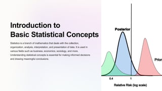
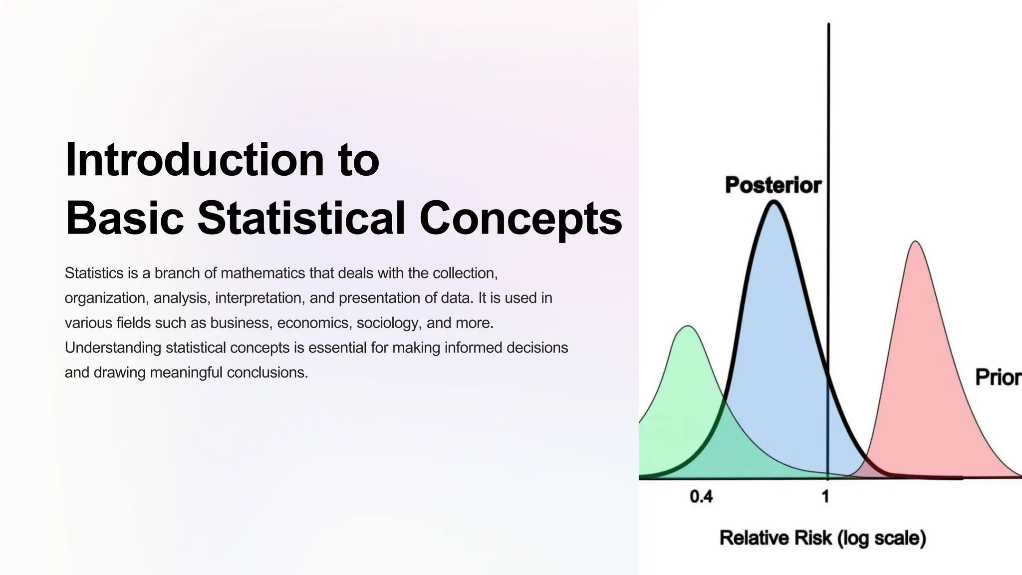
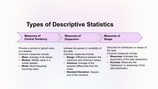
The document provides an overview of basic statistical concepts, including descriptive and inferential statistics, measures of central tendency and variability, as well as sampling methods and common statistical distributions. It emphasizes the importance of understanding these concepts for data analysis and informed decision-making. Key methods and formulas for calculating various statistics such as mean, median, mode, variance, and standard deviation are also discussed.
![Measures of Central Tendency
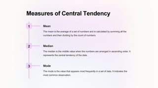
Mean
The mean is the average of a set of numbers, calculated by adding all the numbers together and then dividing by the count of numbers.
Consider the following dataset:
[10, 15, 20, 25, 30]
• (10 + 15 + 20 + 25 + 30) / 5 = 20](https://image.slidesharecdn.com/lect7-240428102444-d2e37880/85/Basic-Statistical-Concepts-in-Machine-Learning-pptx-14-320.jpg)
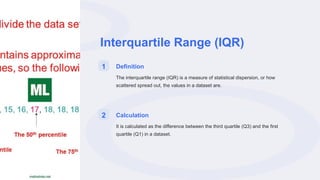
![Measures of Central Tendency
Median
The median is the middle value of a data set when it is ordered from least to greatest. It represents the 50th
percentile of the data.
Consider the following dataset:
[10, 15, 20, 25, 30]
• The Middle value, which is also 20.](https://image.slidesharecdn.com/lect7-240428102444-d2e37880/85/Basic-Statistical-Concepts-in-Machine-Learning-pptx-15-320.jpg)
![Measures of Central Tendency
Mode
The mode is the value that appears most frequently in a given data set. It's the most common observation in the
data.
Consider the following dataset:
[10, 15, 20, 25, 30]
• No Mode in this case.](https://image.slidesharecdn.com/lect7-240428102444-d2e37880/85/Basic-Statistical-Concepts-in-Machine-Learning-pptx-16-320.jpg)
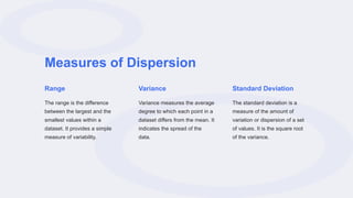
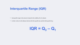
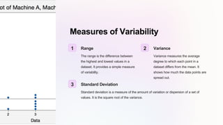
![Measures of Dispersion
Example:
Indicate the spread or variability of the data.
Consider two datasets:
• Dataset A: [5,5,5,5,5]
• Dataset B: [0,10,0,10,0]
• Both datasets have the same mean (5), but Dataset B has higher dispersion.](https://image.slidesharecdn.com/lect7-240428102444-d2e37880/85/Basic-Statistical-Concepts-in-Machine-Learning-pptx-18-320.jpg)
![Measures of Shape
Example:
Describe the distribution or shape of the data.
Consider two datasets:
• Dataset C: [10,15,20,25,30]
• Dataset D: [10,10,20,30,30]
• Both datasets have the same mean and median, but Dataset C is symmetric, while Dataset D is
skewed.](https://image.slidesharecdn.com/lect7-240428102444-d2e37880/85/Basic-Statistical-Concepts-in-Machine-Learning-pptx-19-320.jpg)