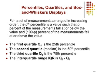
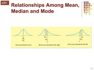
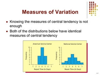
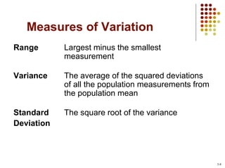
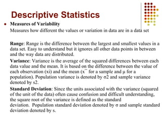
This document provides an introduction to key concepts in statistics including measures of central tendency, variation, distributions, and linear regression. It defines the mean, median, and mode as measures of central tendency. Measures of variation described include range, variance, and standard deviation. Common distributions like the normal distribution are explained and its key properties outlined. Hypothesis testing and p-values are also introduced. Finally, the concepts of covariance, correlation, and simple linear regression models are summarized.

1. Introduction to Statistics
for Business Analytics

2. The Mean
Population X1, X2, …, XN
m
Population Mean
N
X
N
=1
i
i



Sample x1, x2, …, xn
Sample Mean
x
n
x
x
n
=1
i
i


3-2

3. The Sample Mean
and is a point estimate of the population mean
n
x
x
x
n
x
x n
n
i
i






 ...
2
1
1
For a sample of size n, the sample mean (x) is defined as
3-3
Population mean (μ) is average of the population measurements

4. Descriptive Statistics
Measures of Location or measures of central tendency
These measures are summary statistics that represent the
center point or typical value of data
 Mean (Arithmetic Mean): The most used measure of location
is the mean (arithmetic mean) or average value.
 Median: The median is the value in the middle when the data
are arranged in ascending order. It is the middle value, for an
odd number of data and it is the average of two middle values
for an even number of observations.
 Mode: The mode is the value that occurs most frequently in a
data set. If all the data points have a frequency of one, there is
no mode. If the greatest frequency occurs at two or more
different values, there is more than one mode.

5. Properties of the Normal
Distribution
 The shape of any individual normal curve depends on its
specific mean  and standard deviation s
 The highest point is over the mean
 Mean = median = mode
 All measures of central tendency equal each other
 The curve is symmetrical about its mean
 The left and right halves of the curve are mirror
images
6-5

6. Relationships Among Mean,
Median and Mode
LO1
3-6

7. Measures of Variation
 Knowing the measures of central tendency is not
enough
 Both of the distributions below have identical
measures of central tendency
3-7

8. Measures of Variation
Range Largest minus the smallest
measurement
Variance The average of the squared deviations
of all the population measurements from
the population mean
Standard The square root of the variance
Deviation
3-8

9. Descriptive Statistics
 Measures of Variability
Measures how different the values or variation in data are in a data set
Range: Range is the difference between the largest and smallest values in a
data set. Easy to understand but it ignores all other data points in between
and the way data are distributed.
Variance: Variance is the average of the squared differences between each
data value and the mean. It is based on the difference between the value of
each observation (xi) and the mean (x¯ for a sample and μ for a
population). Population variance is denoted by σ2 and sample variance
denoted by s2.
Standard Deviation: Since the units associated with the variance (squared
of the unit of the data) often cause confusion and difficult understanding,
the square root of the variance is defined as the standard
deviation. Population standard deviation denoted by σ and sample standard
deviation denoted by s.

10. Hypothesis
 The null hypothesis and alternative hypotheses are
statements regarding the differences or effects that
occur in the population.
 The null hypothesis assumes that whatever you are
trying to prove did not happen.
 Null Hypotheses (H0): Undertaking seminar classes has
no effect on students' performance.
 Alternative Hypothesis (HA): Undertaking seminar
class has a positive effect on students' performance.
 significance levels to find evidence for either the null or
alternative hypothesis

11. P-value
 Also known as level of significance
 Accepted p – value is 0.05
 If p-value is 0.03 (i.e., p = .03), this means that
there is a 3% chance of finding a difference as
large as (or larger than) the one in your study
given that the null hypothesis is true.

12. Distribution Shapes
 Symmetrical and rectangular
 The uniform distribution
 Symmetrical and bell-shaped
 The normal distribution
 Skewed
 Skewed either left or right
6-12

13. Normal curve
 is a bell-shaped curve which shows the
probability distribution of a continuous
random variable
 represents the distribution of values,
frequencies, or probabilities of a set of data.
6-13

14. The Normal Probability
Distribution Continued
 The normal curve is symmetrical
about its mean 
 The mean is in the middle under the
curve
 So  is also the median
 It is tallest over its mean 
 The area under the entire normal
curve is 1
 The area under either half of the curve
is 0.5
6-14

15. Properties of the Normal
Distribution
 The shape of any individual normal curve depends
on its specific mean  and standard deviation s
 The highest point is over the mean
 Mean = median = mode
 All measures of central tendency equal each other
 The curve is symmetrical about its mean
 The left and right halves of the curve are mirror images
6-15

16. Properties of the Normal
Distribution Continued
 The tails of the normal extend to infinity in
both directions
 The tails get closer to the horizontal axis but
never touch it
 The area under the normal curve to the right
of the mean equals the area under the
normal to the left of the mean
 The area under each half is 0.5
6-16

17. Three Important
Percentages
6-17

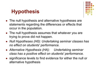
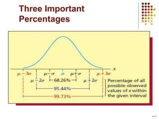
18. The Empirical Rule for
Normal Populations
 If a population has mean µ and standard
deviation σ and is described by a normal
curve, then
 68.26% of the population measurements lie within
one standard deviation of the mean: [µ-σ, µ+σ]
 95.44% of the population measurements lie within
two standard deviations of the mean: [µ-2σ, µ+2σ]
 99.73% of the population measurements lie within
three standard deviations of the mean: [µ-3σ,
µ+3σ]
3-18

19. Percentiles, Quartiles, and Box-
and-Whiskers Displays
For a set of measurements arranged in increasing
order, the pth percentile is a value such that p
percent of the measurements fall at or below the
value and (100-p) percent of the measurements fall
at or above the value
 The first quartile Q1 is the 25th percentile
 The second quartile (median) is the 50th percentile
 The third quartile Q3 is the 75th percentile
 The interquartile range IQR is Q3 - Q1
3-19

20. Five Number Summary
1. The smallest
measurement
2. The first quartile, Q1
3. The median, Md
4. The third quartile, Q3
5. The largest
measurement
 Displayed visually
using a box-and-
whiskers plot
3-20

21. Box-and-Whiskers Plots
 The box plots the:
 First quartile, Q1
 Median, Md
 Third quartile, Q3
 Inner fences
 Outer fences
 Inner fences
 Located 1.5IQR away
from the quartiles:
 Q1 – (1.5  IQR)
 Q3 + (1.5  IQR)
 Outer fences
 Located 3IQR away
from the quartiles:
 Q1 – (3  IQR)
 Q3 + (3  IQR)
3-21

22. Box-and-Whiskers Plots Continued
 The “whiskers” are dashed lines that plot the
range of the data
 A dashed line drawn from the box below Q1 down
to the smallest measurement
 Another dashed line drawn from the box above Q3
up to the largest measurement
3-22

23. Outliers
 Outliers are measurements that are very
different from other measurements
 They are either much larger or much smaller than
most of the other measurements
 Outliers lie beyond the fences of the box-and-
whiskers plot
 Measurements between the inner and outer
fences are mild outliers
 Measurements beyond the outer fences are
severe outliers
3-23

24. Covariance
 A measure of the strength of a linear
relationship is the covariance
 A positive covariance indicates a positive
linear relationship between x and y
 As x increases, y increases
 A negative covariance indicates a negative
linear relationship between x and y
 As x increases, y decreases
3-24

25. Correlation Coefficient
 Magnitude of covariance does not indicate
the strength of the relationship
 Magnitude depends on the unit of measurement
used for the data
 Correlation coefficient (r) is a measure of the
strength of the relationship that does not
depend on the magnitude of the data
y
x
xy
s
s
s
r 
3-25

26. Correlation Coefficient Continued
 Sample correlation coefficient r is always
between -1 and +1
 Values near -1 show strong negative correlation
 Values near 0 show no correlation
 Values near +1 show strong positive correlation
3-26

27. Different Values of the
Correlation Coefficient
13-27

28. The Simple Linear Regression
Model and the Least Squares
Point Estimates
 The dependent (or response) variable is the
variable we wish to understand or predict
 The independent (or predictor) variable is the
variable we will use to understand or predict the
dependent variable
 Regression analysis is a statistical technique that
uses observed data to relate the dependent variable
to one or more independent variables
 The objective is to build a regression model that can
describe, predict and control the dependent variable
based on the independent variable
13-28

29. Form of The Simple Linear
Regression Model
 y = β0 + β1x + ε
 y = β0 + β1x + ε is the mean value of the dependent
variable y when the value of the independent
variable is x
 β0 is the y-intercept; the mean of y when x is 0
 β1 is the slope; the change in the mean of y per unit
change in x
 ε is an error term that describes the effect on y of all
factors other than x
13-29

30. Regression Terms
 β0 and β1 are called regression parameters
 β0 is the y-intercept and β1 is the slope
 We do not know the true values of these
parameters
 So, we must use sample data to estimate
them
 b0 is the estimate of β0 and b1 is the estimate
of β1
13-30

31. The Simple Linear Regression
Model Illustrated
13-31

32. Simple Coefficient of
Determination and Correlation
 How useful is a particular regression model?
 One measure of usefulness is the simple
coefficient of determination
 It is represented by the symbol r2
13-32

33. Calculating The Simple
Coefficient of Determination
1. Total variation is given by the formula
(yi-ȳ)2
2. Explained variation is given by the formula (ŷi-
ȳ)2
3. Unexplained variation is given by the formula (yi-
ŷ)2
4. Total variation is the sum of explained and
unexplained variation
5. r2 is the ratio of explained variation to total
variation
13-33

34. The Multiple Regression Model
 Simple linear regression used one independent
variable to explain the dependent variable
 Some relationships are too complex to be described using
a single independent variable
 Multiple regression uses two or more independent
variables to describe the dependent variable
 This allows multiple regression models to handle more
complex situations
 There is no limit to the number of independent variables a
model can use
 Multiple regression has only one dependent variable
14-34

35. The Multiple Regression
Model
• The linear regression model relating y to x1, x2,…, xk is y =
β0 + β1x1 + β2x2 +…+ βkxk + 
• µy = β0 + β1x1 + β2x2 +…+ βkxk is the mean value of the
dependent variable y when the values of the independent
variables are x1, x2,…, xk
• β0, β1, β2,… βk are unknown the regression parameters
relating the mean value of y to x1, x2,…, xk
•  is an error term that describes the effects on y of all
factors other than the independent variables x1, x2,…, xk
14-35

36. EXAMPLE: The Tasty Sub
Shop Case
14-36

37. Model Assumptions and
the Standard Error
 The model is
y = β0 + β1x1 + β2x2 + … + βkxk + 
 Assumptions for multiple regression are
stated about the model error terms, ’s
14-37

38. R2 and Adjusted R2 Continued
5. The multiple coefficient of determination is
the ratio of explained variation to total
variation
6. R2 is the proportion of the total variation that
is explained by the overall regression model
7. Multiple correlation coefficient R is the
square root of R2
14-38

39. The Adjusted R2
 Adding an independent variable to multiple
regression will raise R2
 R2 will rise slightly even if the new variable has no
relationship to y
 The adjusted R2 corrects this tendency in R2
 As a result, it gives a better estimate of the
importance of the independent variables
14-39