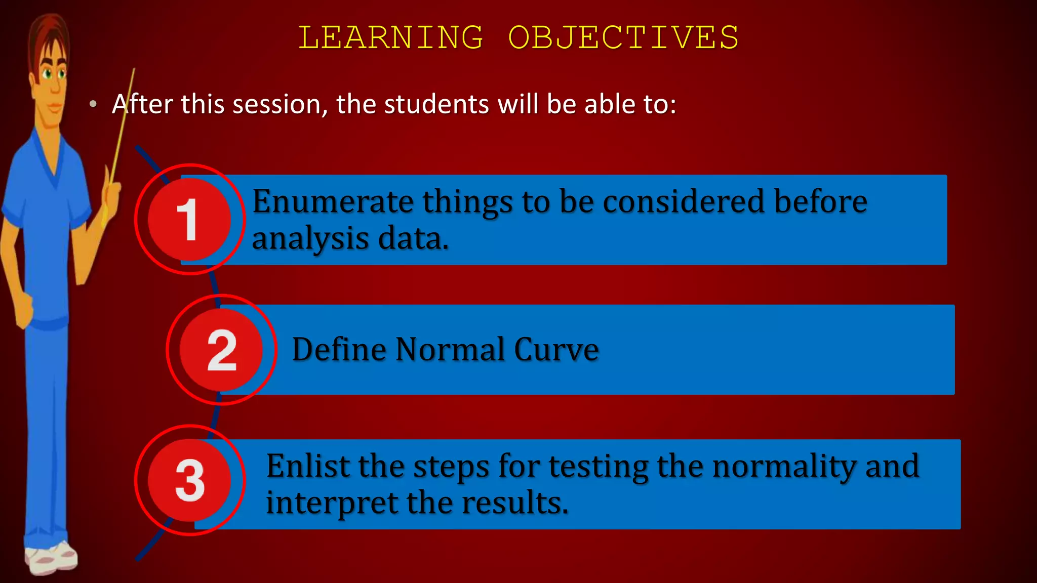
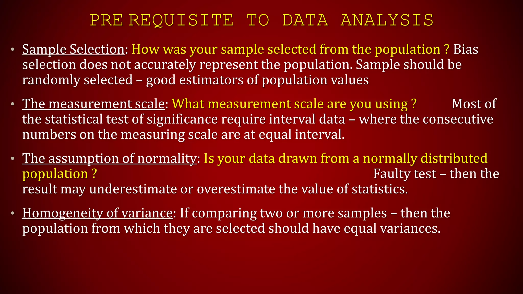
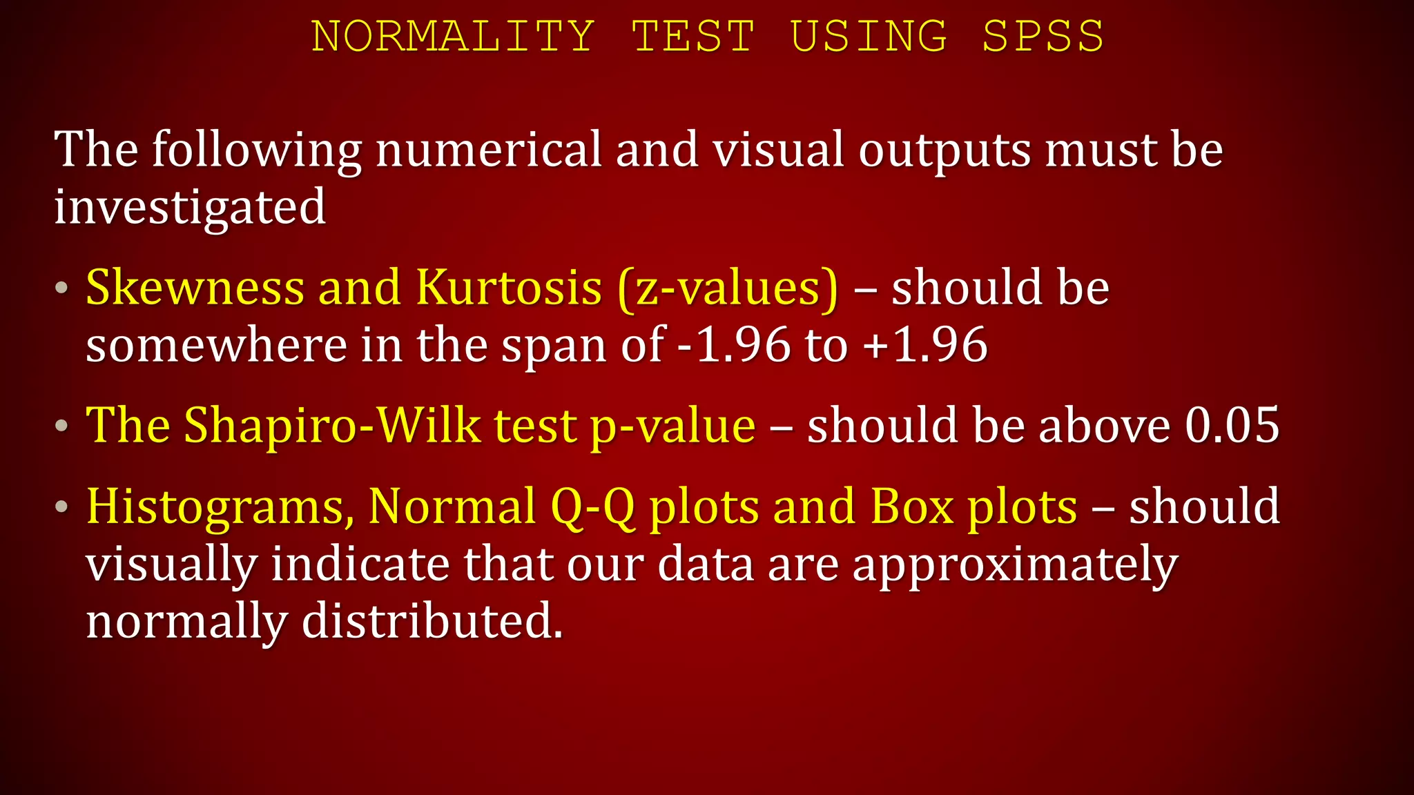
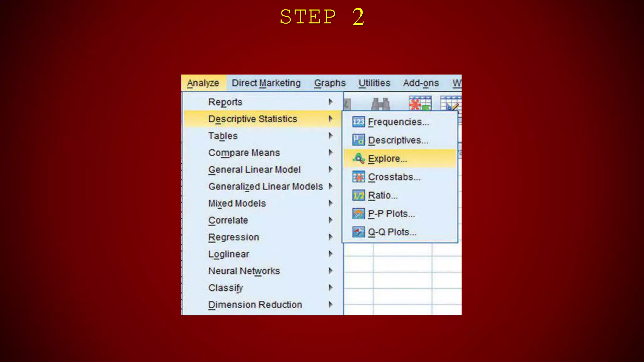
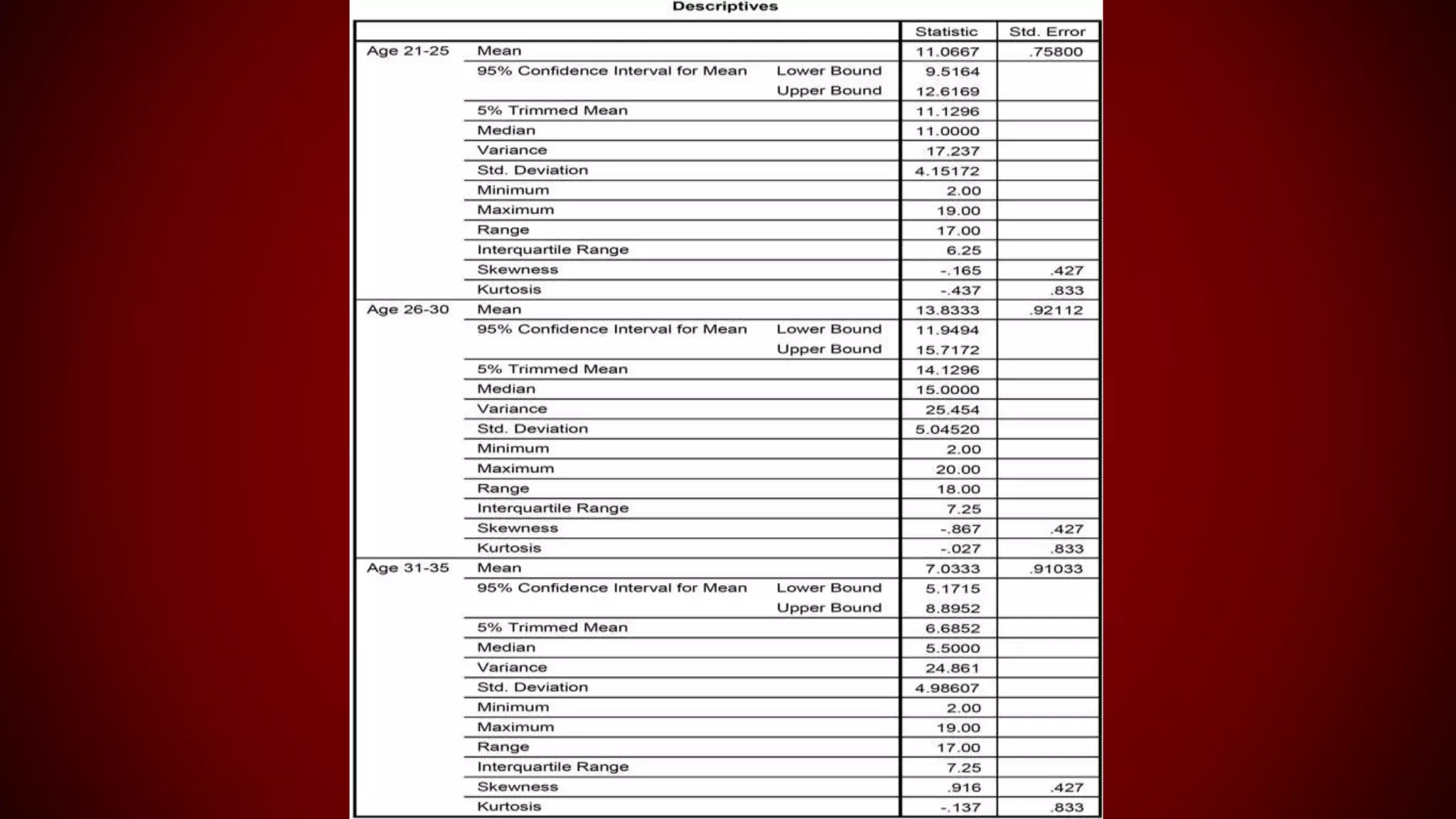
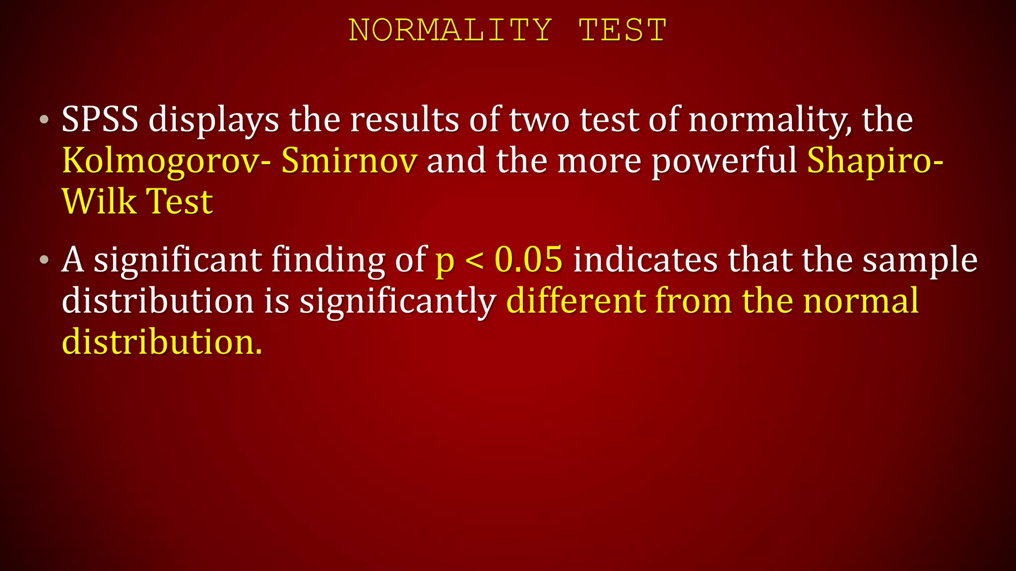
NORMALITY
- NITHIN NAIR (MPT-1)
LEARNING OBJECTIVES
• After this session, the students will be able to:
Enumerate things to be considered before
analysis data.
Define Normal Curve
Enlist the steps for testing the normality and
interpret the results.
PRE REQUISITE TO DATA ANALYSIS
• Sample Selection: How was your sample selected from the population ? Bias
selection does not accurately represent the population. Sample should be
randomly selected – good estimators of population values
• The measurement scale: What measurement scale are you using ? Most of
the statistical test of significance require interval data – where the consecutive
numbers on the measuring scale are at equal interval.
• The assumption of normality: Is your data drawn from a normally distributed
population ? Faulty test – then the
result may underestimate or overestimate the value of statistics.
• Homogeneity of variance: If comparing two or more samples – then the
population from which they are selected should have equal variances.
NORMAL CURVE
• Gaussian Curve
• Smooth Bell Shaped
• Perfectly symmetrical
• Mean = 0
• Standard deviation = 1
• Mean, Median, Mode all coincide
• Based on an infinitely large number of observations – tails
never touch baseline
NORMALITY TEST USING SPSS
The following numerical and visual outputs must be
investigated
• Skewness and Kurtosis (z-values) – should be
somewhere in the span of -1.96 to +1.96
• The Shapiro-Wilk test p-value – should be above 0.05
• Histograms, Normal Q-Q plots and Box plots – should
visually indicate that our data are approximately
normally distributed.
TESTING FOR NORMALITY
• Step 1 – Data Entry
• Step 2 – From Analyze drop-down menu, select
Descriptive Statistics and then Explore.
• Step 3 – Select variables and send them to Dependent List
box.
• Step 4 – Click on the Plots options. Untick Stem and leaf
and tick Histogram and Normality plots with tests
• Step 5 – Click Continue and the Click OK
STEP 1
STEP 2
STEP 3
STEP 4
SPSS OUTPUT
• Look at the values of Skewness and Kurtosis
• Test of Normality Table
• Histogram
• Q-Q Plot
• Box and Whisker Plots
SKEWNESS AND KURTOSIS
• A measure of how far skew and kurtosis deviate from the
normal distribution is found by dividing the value of
skew by the standard error of skew, and by dividing
kurtosis by the standard error of kurtosis.
• If either or both these values is (above +1.96 or below -
1.96), then the assumption of normality is rejected.
NORMALITY TEST
• SPSS displays the results of two test of normality, the
Kolmogorov- Smirnov and the more powerful Shapiro-
Wilk Test
• A significant finding of p < 0.05 indicates that the sample
distribution is significantly different from the normal
distribution.
RESULTS (SAMPLE CHARACTERISTICS)
• A Shapiro-Wilk test (p - ?) and a visual inspection of their
histograms, Q-Q plots and box plots showed that the
given data were / were not normally distributed with a
skewness of (statistical value with SE) and a kurtosis
(statistical value with SE)
REFERENCES
• Foundations of Clinical Research – Leslie G Portney (3rd ed)
• Confidence in Community Medicine – Ebrahim Patel (3rd ed)
• SPSS Explained – Perry R Hinton (2nd ed)
• Research Methodology – CR Kothari (3rd ed)
• Methods in Biostatistics – BK Mahajan (7th ed)
Normality

Normality

  • 1.
  • 2.
    LEARNING OBJECTIVES • Afterthis session, the students will be able to: Enumerate things to be considered before analysis data. Define Normal Curve Enlist the steps for testing the normality and interpret the results.
  • 3.
    PRE REQUISITE TODATA ANALYSIS • Sample Selection: How was your sample selected from the population ? Bias selection does not accurately represent the population. Sample should be randomly selected – good estimators of population values • The measurement scale: What measurement scale are you using ? Most of the statistical test of significance require interval data – where the consecutive numbers on the measuring scale are at equal interval. • The assumption of normality: Is your data drawn from a normally distributed population ? Faulty test – then the result may underestimate or overestimate the value of statistics. • Homogeneity of variance: If comparing two or more samples – then the population from which they are selected should have equal variances.
  • 4.
    NORMAL CURVE • GaussianCurve • Smooth Bell Shaped • Perfectly symmetrical • Mean = 0 • Standard deviation = 1 • Mean, Median, Mode all coincide • Based on an infinitely large number of observations – tails never touch baseline
  • 5.
    NORMALITY TEST USINGSPSS The following numerical and visual outputs must be investigated • Skewness and Kurtosis (z-values) – should be somewhere in the span of -1.96 to +1.96 • The Shapiro-Wilk test p-value – should be above 0.05 • Histograms, Normal Q-Q plots and Box plots – should visually indicate that our data are approximately normally distributed.
  • 6.
    TESTING FOR NORMALITY •Step 1 – Data Entry • Step 2 – From Analyze drop-down menu, select Descriptive Statistics and then Explore. • Step 3 – Select variables and send them to Dependent List box. • Step 4 – Click on the Plots options. Untick Stem and leaf and tick Histogram and Normality plots with tests • Step 5 – Click Continue and the Click OK
  • 7.
  • 8.
  • 9.
  • 10.
  • 11.
    SPSS OUTPUT • Lookat the values of Skewness and Kurtosis • Test of Normality Table • Histogram • Q-Q Plot • Box and Whisker Plots
  • 13.
    SKEWNESS AND KURTOSIS •A measure of how far skew and kurtosis deviate from the normal distribution is found by dividing the value of skew by the standard error of skew, and by dividing kurtosis by the standard error of kurtosis. • If either or both these values is (above +1.96 or below - 1.96), then the assumption of normality is rejected.
  • 15.
    NORMALITY TEST • SPSSdisplays the results of two test of normality, the Kolmogorov- Smirnov and the more powerful Shapiro- Wilk Test • A significant finding of p < 0.05 indicates that the sample distribution is significantly different from the normal distribution.
  • 19.
    RESULTS (SAMPLE CHARACTERISTICS) •A Shapiro-Wilk test (p - ?) and a visual inspection of their histograms, Q-Q plots and box plots showed that the given data were / were not normally distributed with a skewness of (statistical value with SE) and a kurtosis (statistical value with SE)
  • 21.
    REFERENCES • Foundations ofClinical Research – Leslie G Portney (3rd ed) • Confidence in Community Medicine – Ebrahim Patel (3rd ed) • SPSS Explained – Perry R Hinton (2nd ed) • Research Methodology – CR Kothari (3rd ed) • Methods in Biostatistics – BK Mahajan (7th ed)