The document is a lab report submitted by Mr. Yuvraj Singh for his Control System Lab course. It includes an index listing 8 experiments performed, along with the objectives, requirements, theory, programs, outputs, and results for Experiment 1 on introducing MATLAB software and Experiment 2 on obtaining a transfer function from zero-pole-gain parameters in MATLAB. The experiments involve modeling and analyzing first and second order control systems using MATLAB.

1. Mr. Yuvraj Singh 1
GLOBAL TECHNICAL CAMPUS
A
LAB REPORT
OF
CONTROL SYSTEM LAB (6EE7A)
2016-2017
Submitted To Submitted By
Mr. Rajeev Kumar Mr. Yuvraj Singh
A.P. Dept. of EE 14EGCEE037
DEPARTMENT OF ELECTRICAL ENGINEERING
GLOBAL INSTITUTE OF TECHNOLOGY, JAIPUR
ITS-1&2, IT PARK, EPIP, SITAPURA, JAIPUR, 302022 (RAJ.)

2. Mr. Yuvraj Singh 2
INDEX
S.No. Name of Experiment Date of
Performance
Date of
Submission
Teacher’s
Signature
Remark
1 Introduction of
MATLAB Computing
Control Software.
18/01/17 25/01/17
2 Using MATLAB obtain
transfer function when
ZPK are given
18/01/17 25/01/17
3 Using Matlab obtain
Transfer function when
coefficient of S are
given.
25/01/17 01/02/17
4 Study and plot Step
response of First order
control system using
MATLAB.
01/02/17 08/02/17
5 Study and Plot Time
Responce of 2nd
order for
given conditions.
A. Un-Damped
B. Under Damped
C. Critical Damped
D. Over Damped
08/02/17 15/02/17
6 Study and Plot Transfer
Responce of 2nd order
System for Under
Damped conditions.
1. Rise Time
2. Delay Time
3. Peak Time
4. Max. OverShoot
5. Stalling Time with 2%
Error
6. Stalling Time with 5%
Error
15/02/17 21/03/17
7 Study 1st
order RC N/W
obtain TF and plot
step,impulse and ramp
response
21/03/17 05/04/17
8 Study RLC Series N/W
obtain TF and plot step
and ramp response
05/04/17 16/05/17

3. Mr. Yuvraj Singh 3
EXPERIMENT NO. 1
OBJECT:- Introduction of MATLAB Computing Control Software.
REQUREMENT:- MATLAB (R 2008a) Software.
THEORY
MATLAB is a high performance language for technical computation. It integrate
computation, visualization and programming in a way to use environment where problem and
solution are expressed in a family mathematic notation. MATLAB is widely used in all areas of
applied mathematics, in education and research at universities, and in the industry.This makes
the software particularly useful for linear algebra but MATLAB is also a great tool for solving
algebraic and differential equations and for numerical integration. MATLAB has powerful
graphic tools and It is also a programming language, and is one of the easiest programming
languages for writing mathematical programs.
The MATLAB consists of the following topics:
 The MATLAB Environment
 Using the Help System in MATLAB
 MATLAB Basics
 Linear Algebra; Vectors and Matrices
 M files; Scripts and User-defined functions
 Plotting
 Flow Control and Loops; For and While Loops, If and Case statements
 Mathematics and Computation
 Algorithm Development
 Data Equitation
 Modeling Simulation and Prototyping

4. Mr. Yuvraj Singh 4
System Parts:- The MATLAB lab system is consist the following Five main parts.
1. Development Environment:-
This is set of tools and functionalities that help you to use MATLAB function and files.
2. MATLAB Mathematical Function Theory:-
This is the best collection of computational algorithm manging from elemantry function like
Sum,Sine and Complex algorithm.
3. MATLAB Language:-
This is high level matrix array language with control flow Statements, Function, Data, Structure
I/p & O/p and Object Programing.
4. Graphics:-
MATLAB has extensive facilities for displaying vectors and matrix as graph as well as
annotating and printing these graphs.
5. MATLAB Application Program Interface:-
This is library that allow you to interfaced with MATLAB.
The MATLAB Environment consists of the following main parts:
• Command Window
• Command History
• Workspace
• Current Folder
• Editor

5. Mr. Yuvraj Singh 5
1. Command Window
The Command Window is the main window in MATLAB. Use the Command Window to enter
variables and to run functions and M-files scripts (more about m-files later).
2. Command History
Statements you enter in the Command Window are logged in the Command History. From the
Command History, you can view and search for previously run statements, as well as copy and
execute selected statements. You can also create an M-file from selected statements.

6. Mr. Yuvraj Singh 6
3. Workspace
The WorkSpace window list all your variables used as long you have MATLAB opened.You
may also save all your variables and data to a text file (.mat file), this is useful if you want to
save your data and use it for later. You could also use the following command
>>who:- This command list all the commands used.
>>whos:- This command lists all the command with the current values, dimensions, etc.
>>clear:- This command will clear all the variables in your workplace.
4. Current Folder
The ―Current Folder‖ window lists all m files, etc. available in the current directory. You
should set your working folder as the Current Directory or set your working folder as part of the
search path, if you don’t MATLAB will not find your files.
5. Editor
The Editor is used to create scripts and m-files. Click the ―New Script‖ button in the Toolbar.
When you learn about m-files (scripts and functions) in a later chapter you will be using this
editor to enter your commands and save them.

7. Mr. Yuvraj Singh 7
 Linear Algebra
Linear Algebra is a branch of mathematics concerned with the study of matrices, vectors, vector
spaces (also called linear spaces), linear maps (also called linear transformations), and systems of
linear equations.Some useful functions for Linear Algebra in MATLAB.
 The COLON Operator:- The colon (;) is one of the most important symbol for the
MATLAB programming. It occurs in general different form. The colon operator is one
way of creating long vectors that are useful for indexing (see the next section).The colon
operator produces a row vector starting with the first argument and incrementing by one
until the second argument has been reached.
Result:- We have successfully study of the Introduction of MATLAB Computing Control
Software.

8. Mr. Yuvraj Singh 8
EXPERIMENT - 2
OBJECT:- Using MATLAB obtain transfer function when ZPK are given.
REQUIRMENTS:- MATLAB 7.6.0 (R2008a), computer system.
THEORY
A Transfer Function is the ratio of the output of system to the input of a system, in
the laplace domain considering its initial conditions and equilibrium point to be zero. This
assumption is relaxed for systems observing translence. If we have an input function of X(s), and
an output function Y(s), we define the transfer function H(s) to be: H(s)= Y(s)/X(s).
POLES and ZEROS
Poles and Zeros of a transfer function are the frequencies for which the value of
the denominator and numerator of transfer function becomes zero respectively. The values of the
poles and the zeros of a system determine whether the system is stable, and how well the system
performs. Control systems, in the most simple sense, can be designed simply by assigning
specific values to the poles and zeros of the system.
Effects of Poles and Zeros
As S approaches a zero, the numerator of the transfer function (and therefore the
transfer function itself) approaches the value 0. When s approaches a pole, the denominator of
the transfer function approaches zero, and the value of the transfer function approaches infinity.
An output value of infinity should raise an alarm bell for people who are familiar with BIBO
stability. We will discuss this later.
As we have seen above, the locations of the poles, and the values of the real and imaginary parts
of the pole determine the response of the system. Real parts correspond to exponentials, and
imaginary parts correspond to sinusoidal values. Addition of poles to the transfer function has
the effect of pulling the root locus to the right, making the system less stable.

9. Mr. Yuvraj Singh 9
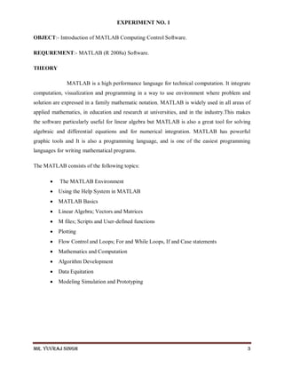
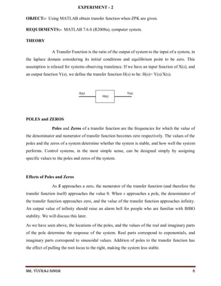
Creation of Zero-Pole-Gain Models
sys = zpk(Z,P,K) creates a continuous-time zero-pole-gain model with zeros Z,
poles P, and gain(s) K. The output sys is a zpk model object storing the model data.
In the SISO case, Z and P are the vectors of real- or complex-valued zeros and poles, and K is
the real- or complex-valued scalar gain:
h(s)=k(s−z(1))(s−z(2))…(s−z(m))(s−p(1))(s−p(2))…(s−p(n))
Set Z or p to [] for systems without zeros or poles. These two vectors need not have equal
length and the model need not be proper (that is, have an excess of poles).
To create a MIMO zero-pole-gain model, specify the zeros, poles, and gain of each SISO
entry of this model. In this case:
 Z and P are cell arrays of vectors with as many rows as outputs and as many columns as
inputs, and K is a matrix with as many rows as outputs and as many columns as inputs.
 The vectors Z{i,j} and P{i,j} specify the zeros and poles of the transfer function from
input j to output i.
 K(i,j) specifies the (scalar) gain of the transfer function from input j to output i.
PROGRAM
Z=[-1,-2];
P=[1,2,-3];
K=[37];
t=zpk(Z,P,K)
OUTPUT
Zero/pole/gain:
37 (s+1) (s+2)
-----------------
(s-1) (s-2) (s+3)
RESULT:- We have successfully execute the program in ZPK form.

10. Mr. Yuvraj Singh 10
EXPERIMENT NO. 3
OBJECT:- Using Matlab obtain Transfer function when coefficient of S are given.
REQUIRMENTS:- MATLAB 7.6.0 (R2008a), computer system.
THEORY
A Transfer Function is the ratio of the output of system to the input of a system, in
the laplace domain considering its initial conditions and equilibrium point to be zero. This
assumption is relaxed for systems observing translence. If we have an input function of X(s), and
an output function Y(s), we define the transfer function H(s) to be: H(s)= Y(s)/X(s).
Step Response
Similar to the impulse response, the step response of a system is the output of the
system when a unit step function is used as the input. The step response is a common analysis
tool used to determine certain metrics about a system. Typically, when a new system is designed,
the step response of the system is the first characteristic of the system to be analyzed.
Poles and Zeros
Poles and Zeros of a transfer function are the frequencies for which the value of
the denominator and numerator of transfer function becomes zero respectively. The values of the
poles and the zeros of a system determine whether the system is stable, and how well the system
performs. Control systems, in the most simple sense, can be designed simply by assigning
specific values to the poles and zeros of the system.
• Laplace Transforms useful for describing systems – Differential equations→algebraic
equations – Convolution→multiplication
• For LTI (linear-time-invariant) systems input-output relationship:
Y (s) = G(s)U(s)
G(s) =n(s) d(s)

11. Mr. Yuvraj Singh 11
Transfer function
• The transfer function describes how the input (in the Laplace domain) is transferred to the
output (in the Laplace domain).
• The transfer function does not give explicit information about initial conditions It gives an easy
way to compute the forced response
• G(s) = L−1
{g(t)} where g(t) is the impulse response of G.
Poles and zeros
• Transfer function G(s) contains information through its poles and zeros
• Typical transfer function:
G(s) =n(s) d(s)
Values of s such that n(s) = 0 - zeros
Values of s such that d(s) = 0 - poles
i.e. G(s) = 0 when n(s) = 0 and G(s) = ∞when d(s) = 0
Poles and Stability:-
• Consider a first order system with transfer function G(s) = 1 s + a , a > 0 • Inverse Laplace
transform (impulse response) therefore is g(t) = e−at
Thus response to impulse gradually decays.
• Consider a first order system with transfer function G(s) = 1 s−a , a > 0 • Inverse Laplace
transform (impulse response) therefore is g(t) = e^aT
Thus response to impulse gradually grows exponentially.

12. Mr. Yuvraj Singh 12
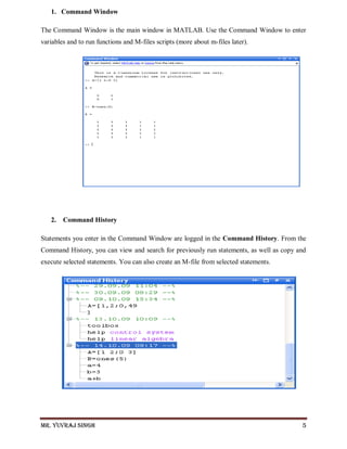
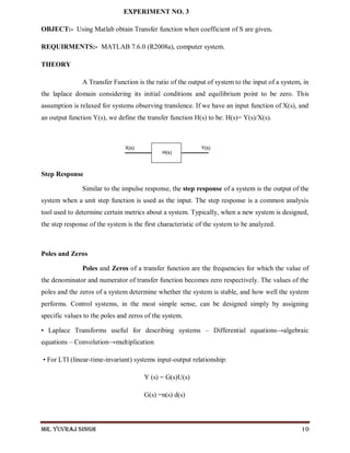
PROGRAM
N=[k,3*k,2*k];
D=[1,0,-7,6];
K=37;
T=tf(N,D)
OUTPUT
K = 37
N = 37 111 74
D = 1 0 -7 6
Transfer function
37 s^2 + 111 s + 74
------------------
s^3 - 7 s + 6
RESULT:- We have successfully excute the transfer function when coefficient of S are given.

13. Mr. Yuvraj Singh 13
EXPERIMENT NO. 4
OBJECT:- Study and plot Step response of First order control system using MATLAB.
REQUIRMENT:- MATLAB 7.6.0 (R2008a), computer system.
THEORY
Transfer Function:- It is defined as the ratio of output and input.
Poles of a Transfer Function
The poles of transfer function are the value of Laplace Transform variable(s), that
cause the transfer function becomes infinite
The denominator of a transfer function is actually the poles of function.
Zeros of a Transfer Function
The zeros of transfer function are the values of Laplace Transform variable(s),
that cause the transfer function becomes zero
The nominator of a transfer function is actually the zeros of function.
First Order Control System
There are two methods to controlling systems. One is open loop system and other
is feedback control system. In open loop system, input proceed to the given process and produces
output. There is no feedback which tells whether desired output comes or not. Other is feedback
control system which has the ability to check whether desired output achieved and if not, it gives
feedback to the controller who controls the system. If the input is unit step, the output is step
response.
The step response yields a clear vision of the system’s transient response. We have two types of
system, first order system and second order system, which are representative of many physical
systems. First order of system is defined as first derivative with respect to time and second order
of system is second derivative with respect to time.
The forced response is also called the steady state response or particular equation. The natural
response is also called the homogeneous equation.

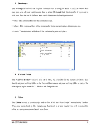
14. Mr. Yuvraj Singh 14
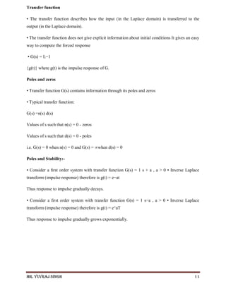
Here we discuss the first order control system without zeros. First order control
system tell us the speed of the response that what duration it reaches to the steady state.
If the input is unit step, R(s) = 1/s so the output is step response C(s). The general equation of 1st
order control system is
C(s) = R(s)G(s)
i.e
C(s) = a/s(s + a)and G(s) is transfer function.
There are two poles, one is input pole at the origin s = 0 and other is system pole at s = -a, this
pole is at negative axis of pole plot. We can find the pole and zeros in MATLAB SOFTWARE
by using command pzmap means pol zero map.
We now taking the inverse transform so total response is becomes y(t) = cf(t) + cn(t) which is
sum of forced response and natural response. Due to the input pole at the origin.
A. Impluse Response Of 1st
Order System
PROGRAM
A=37;
N=[1];
D=[A,1];
T=tf(N,D)
impulse(T)
grid on
OUTPUT
Transfer Function
1
-------
3 7s + 1

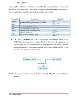
15. Mr. Yuvraj Singh 15
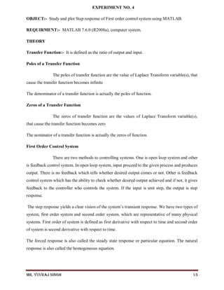
Graph-
Fig:- Impluse Response Of 1st
Order System
B. Step Response Of 1st
Order System
PROGRAM
T=[37]
N=[1]
D=[T,1]
T=tf(N,D)
step(T)
grid on
OUTPUT
T = 37
N = 1
D = 37 1
0 5 10 15 20 25
0
0.05
0.1
0.15
0.2
0.25
0.3
0.35
imp responce of 1st order RC series N/W (37)
Time (sec)
Amplitude

16. Mr. Yuvraj Singh 16
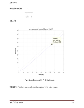
Transfer function 1
-----------
37 s + 1
GRAPH
Fig:- Step Response Of 1st
Order System
C. Ramp Responce Of 1st
Order System
Program
Y=37;
N=[1];
D=[Y,1];
T=tf(N,D)
A=0:0.5:50;
u=A;
lsim(T,U,A)
grid on
Step Response
Time (sec)
Amplitude
0 50 100 150 200 250
0
0.1
0.2
0.3
0.4
0.5
0.6
0.7
0.8
0.9
1
System: T
Time (sec): 37
Amplitude: 0.632
System: T
Time (sec): 74
Amplitude: 0.865
System: T
Time (sec): 148
Amplitude: 0.982

17. Mr. Yuvraj Singh 17
OUTPUT
Transfer function 1
---------------
37 s + 1
GRAPH
Fig:- Ramp Responce Of 1st
Order System
RESULT:- We have successfully plot the response of 1st order system.
0 5 10 15 20 25 30 35 40 45 50
0
5
10
15
20
25
30
35
40
45
50
System: Y
Time (sec): 37
Amplitude: 33.3
ramp responce of 1st order RC series N/W (37)
Time (sec)
Amplitude

18. Mr. Yuvraj Singh 18
EXPERIMENT NO. 5
OBJECT:- Study and Plot Time Responce of 2nd
order for given conditions.
A. Un-Damped B. Under Damped
C. Critical Damped D. Over Damped
REQURIMENT:- MATLAB (R 2008a) Software
THEORY
The order of a control system is determined by the power of s in the denominator
of its transfer function. If the power of s in the denominator of transfer function of a control
system is 2, then the system is said to be 2nd
order control system.
The block diagram of the 2nd
order system
The general expression of transfer function of a 2nd
order control system is given as
Where, ζ= Damping Ratio And ωn=Natural Frequency of the system.
Conditions For The Time Responce of 2nd
order are given as
1. Un-Damped
2. Under Damped
3. Critically Damped
4. Over damped system

19. Mr. Yuvraj Singh 19
1. Un-Damped:- A system is said to be Undamped system when the value of zeta is zero.
No damping occurs in this case.This is also known as Sustained Oscillations. For Un-
Damped conditions the value of ζ=0 .
PROGRAM
ωn=37;
ζ=0;
N=[ωn*ωn]
D=[1,2*ζ*ωn,ωn*ωn]
A=0:0.1:5;
T=tf(N,D)
step(T,A)
title('step response of 2nd order system for undamped condition')
OUTPUT
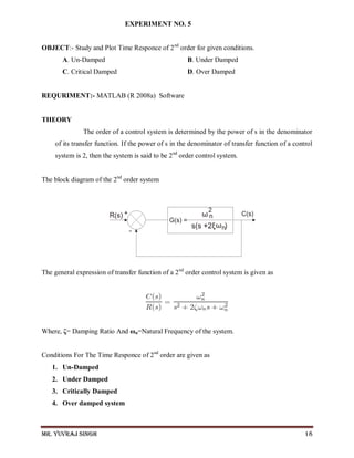
N = 1369
D = 1 0 1369
Transfer function: 1369
-------------------
(s^2 + 1369)

20. Mr. Yuvraj Singh 20
GRAPH
Fig:- Un-Damped Condition
2. Under Damped:- A system is said to be under damped system when the value of ζ is
less than one. In this case roots are complex in nature and the real parts are always
negative. System is asymptotically stable. Rise time is lesser than the other system with
the presence of finite overshoot. For Under Damped conditions the range is 0 < ζ < 1 .
PROGRAM
ωn=37;
ζ=0.3;
N=[ωn*ωn]
D=[1,2*ζ*ωn,ωn*ωn]
T=tf(N,D)
step(T)
title('step response of 2nd order system for under damped condition')
grid on
0 0.5 1 1.5 2 2.5 3 3.5 4 4.5 5
0
0.2
0.4
0.6
0.8
1
1.2
1.4
1.6
1.8
2
step response of 2nd order system for undamped condition
Time (sec)
Amplitude

21. Mr. Yuvraj Singh 21
OUTPUT
N=1369
D =1.0e+003 *
0.0010 0.0222 1.3690
Transfer Function 1369
-------------------------
(s^2 + 22.2 s + 1369)
GRAPH
Fig:- Under Damped Condition
0 0.1 0.2 0.3 0.4 0.5 0.6 0.7 0.8
0
0.2
0.4
0.6
0.8
1
1.2
1.4
step respons of 2nd order systemfor underdamped condition
Time (sec)
Amplitude

22. Mr. Yuvraj Singh 22
3. Critically Damped:- A system is said to be critically damped system when the value of ζ
is one. In this case roots are real in nature and the real parts are always repetitive in
nature. System is asymptotically stable. Rise time is less in this system and there is no
presence of finite overshoot. For Critical Damped conditions the value of ζ =1 .
PROGRAM
ωn=37;
ζ=1;
N=[ ωn*ωn]
D=[1,2* ζ*ωn,ωn*ωn]
T=tf(N,D)
step(T)
title('step response of 2nd order system for critical damped condition')
grid on
OUTPUT
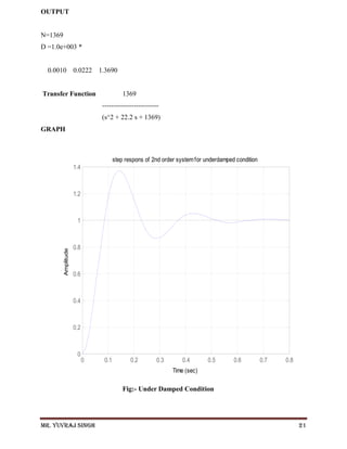
N =1369
D =1 74 1369
Transfer Function: 1369
-----------------------
s^2 + 74 s + 1369

23. Mr. Yuvraj Singh 23
GRAPH
Fig:- Critical Damped Condition
4. Over damped system :- A system is said to be over damped system when the value of ζ is
greater than one. In this case roots are real and distinct in nature and the real parts are always
negative. System is asymptotically stable. Rise time is greater than the other system and there is
no presence of finite overshoot. For Over Damped conditions the range is ζ > 1 .
PROGRAM
ωn=37;
ζ=10;
N=[ ωn*ωn]
D=[1,2* ζ*ωn,ωn*ωn]
T=tf(N,D)
step(T)
title('step response of 2nd order system for overdamped condition')
grid on
0 0.05 0.1 0.15 0.2 0.25 0.3
0
0.1
0.2
0.3
0.4
0.5
0.6
0.7
0.8
0.9
1
step response of 2nd order system for critical damped condition
Time (sec)
Amplitude

24. Mr. Yuvraj Singh 24
OUTPUT
N = 1369
D = 1 740 1369
Transfer Function: 1369
-------------------------
s^2 + 740 s + 1369
GRAPH
Fig:-Over Damped Condition
Result:- We have successfully Study and plote time responce of 2nd
order for given conditions.
A. Un-Damped B. Under Damped
C. Critical Damped D. Over Damped
0 0.5 1 1.5 2 2.5 3 3.5
0
0.1
0.2
0.3
0.4
0.5
0.6
0.7
0.8
0.9
1
step response of 2nd order systemfor overdamped condition
Time (sec)
Amplitude

25. Mr. Yuvraj Singh 25
EXPERIMENT NO. 6
OBJECT:- Study and Plot Transfer Responce of 2nd order System for Under Damped
conditions.
1. Rise Time 2. Delay ime
3. Peak Time 4. Max. OverShoot
5. Stalling Time with 2% Error
6. Stalling Time with 5% Error
REQURIMENT: MATLAB (R 2008a) Software
THEORY
The order of a control system is determined by the power of s in the denominator of
its transfer function. If the power of s in the denominator of transfer function of a control
system is 2, then the system is said to be second-order control system.
The block diagram of the second order system
The general expression of transfer function of a second order control system is given as
Where, ζ= Damping Ratio And ωn=Natural Frequency of the system
1. Peak Time (Tp)
The time required by response to reach its first peak i.e. the peak of first cycle of oscillation,
or first overshoot. On differentiating the expression of c(t) we can obtain the expression for
peak time dc(t)/ dt = 0 .
2. Delay Time (Td)
The time required to reach at 50% of its final value by a time response signal during its first
cycle of oscillation.

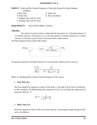
26. Mr. Yuvraj Singh 26
3. Rise Time (Tr)
The time required to rise from 10% to 90% of its final value by a under damped time
response signal during its first cycle of oscillation.
4. Maximum overshoot (Mp)
The difference between the magnitude of the highest peak of time response and magnitude of
its steady state. Maximum overshoot is expressed in term of percentage of steady-state value
of the response.
5. Settling time (Ts)
The time required by the response to reach and steady within specified range of 2 % to 5 % of its
final value. In other words The settling time of a response is that time after which the response
reaches to its steady-state condition with value above nearly 98 % of its final value.
PROGRAM
ωn=37;
ζ =0.3;
N=[ωn*ωn]
D=[1,2*ζ*ωnωn*ωn]
T=tf(N,D)
step(T)
title('step response of 2nd order syste m for under damped condition')
OUTPUT
N=1369
D =1.0e+003 *
0.0010 0.0148 1.3690

27. Mr. Yuvraj Singh 27
Transfer function: 1369
-----------------------
s^2 + 14.8 s + 1369
Observation Table
S.NO. Parameters Practical
values
Theoretial
Values
1. Td 0.0297 Sec 0.047 Sec
2. Tr 0.0332 Sec 0.059 Sec
3. Tp 0.0849 Sec 0.089 Sec
4. Mp 0.526 0.3723
5. Ts 0.5296 Sec 0.360 Sec
Result:- We have successfully Study and Plot Transfer Responce of 2nd order System for
Under Damped conditions.
1. Rise Time 2. Delay Time
3. Peak Time 4. Max. OverShoot
5. Stalling Time with 2% Error
6. Stalling Time with 5% Error
step response of 2nd order systemfor under damped condition
Time (sec)
Amplitude
0 0.1 0.2 0.3 0.4 0.5 0.6 0.7 0.8 0.9
0
0.2
0.4
0.6
0.8
1
1.2
1.4
1.6
System: T
Settling Time (sec): 0.529System: T
Rise Time (sec): 0.0332
System: T
Time (sec): 0.386
Amplitude: 0.98
System: T
Time (sec): 0.372
Amplitude: 0.95
System: T
Peakamplitude: 1.53
Overshoot (%): 52.6
At time (sec): 0.0849
Mp

28. Mr. Yuvraj Singh 28
EXPERIMENT NO. 7
OBJECT:- Study 1st
order RC N/W obtain TF and plot
1. Step Response
2. Impulse Response and
3. Ramp Response
REQURIMENT:- MATLAB (R 2008a) Software
THEORY
There are three basic, linear passive lumped analog circuit components: the
resistor (R) and the capacitor (C). These may be combined in the RC circuit. These circuits,
among them, exhibit a large number of important types of behaviour that are fundamental to
much of analog electronics. In particular, they are able to act as passive filters.
RC CKT in Parallel and Series Combination
The simplest RC circuit is a capacitor and a resistor in parallel. When a circuit
consists of only a charged capacitor and a resistor, the capacitor will discharge its stored energy
through the resistor. The voltage across the capacitor, which is time dependent, can be found by
using Kirchhoff's current law, where the current charging the capacitor must equal the current
through the resistor. When fed by a current source, the transfer function of a parallel and series
RC circuit is:
.
The parallel RC circuit is generally of less interest than the series circuit. This is largely
because the output voltage Voutis equal to the input voltage Vin — as a result, this circuit does not
act as a filter on the input signal unless fed by a current source.

29. Mr. Yuvraj Singh 29
If we have an input function of X(s), and an output function Y(s), we define the
transfer function
H(s) to be: H(s)= Y(s)/X(s).
Having applied the step input and rearranged the equation in the frequency domain, we are now
ready to transform back to the time domain. Checking the Laplace transform tables, a frequency
domain function of the type b/s(s+b) has a time domain equivalent of (1-e-bt
). In the equation
above, b = 1/RC, therefore:
This equation describes the change in voltage across the capacitor when a step input voltage of a
Volts is applied to the circuit.
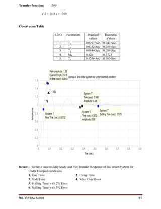
1. Step Response Of 1st
Order RC N/W
PROGRAM
R=37
C=.1
T=R*C
N=[1]
D=[T,1]
A=tf(N,D)
step(A)
grid on
Title ('step responce of 1st order RC series N/W (37)' )

30. Mr. Yuvraj Singh 30
OUTPUT
R = 37
C = 0.1000
T = 3.7000
N = 1
D = 3.7000 1.0000
Transfer function: 1
---------
3.7 s + 1
GRAPH
Fig:- Step Response Of 1st
Order RC N/W
0 5 10 15 20 25
0
0.1
0.2
0.3
0.4
0.5
0.6
0.7
0.8
0.9
1
step responce of 1st order RC series N/W (37)
Time (sec)
Amplitude

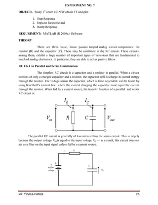
31. Mr. Yuvraj Singh 31
2. Impluse Response Of 1st
Order RC N/W
PROGRAM
R=37
C=.1
T=R*C
N=[1]
D=[T,1]
A=tf(N,D)
impulse(A)
grid on
Title ('imp responce of 1st order RC series N/W (37)' )
OUTPUT
R = 37
C = 0.1000
T = 3.7000
N = 1
D = 3.7000 1.0000
Transfer function: 1
-----------
3.7 s + 1

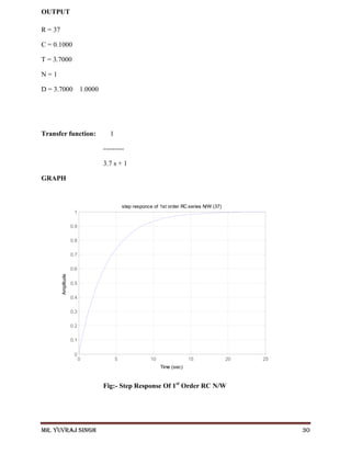
32. Mr. Yuvraj Singh 32
GRAPH
Fig:- Impluse Response Of 1st
Order RC N/W
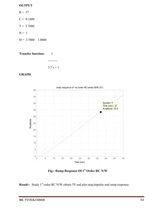
3. Ramp Response Of 1st
Order RC N/W
PROGRAM
R=37
C=.1
T=R*C
N=[1]
D=[T,1]
Y=tf(N,D)
A=0:0.001:50;
U=A;
lsim(Y,U,A)
grid on
Title ('ramp responce of 1st order RC series N/W (37)')
0 5 10 15 20 25
0
0.05
0.1
0.15
0.2
0.25
0.3
0.35
imp responce of 1st order RC series N/W (37)
Time (sec)
Amplitude

33. Mr. Yuvraj Singh 33
OUTPUT
R = 37
C = 0.1000
T = 3.7000
N = 1
D = 3.7000 1.0000
Transfer function: 1
---------
3.7 s + 1
GRAPH
Fig:- Ramp Response Of 1st
Order RC N/W
Result:- Study 1st
order RC N/W obtain TF and plot step,impulse and ramp response.
0 5 10 15 20 25 30 35 40 45 50
0
5
10
15
20
25
30
35
40
45
50
System: Y
Time (sec): 37
Amplitude: 33.3
ramp responce of 1st order RC series N/W (37)
Time (sec)
Amplitude

34. Mr. Yuvraj Singh 34
EXPERIMENT NO. 8
OBJECT:- Study RLC Series N/W obtain TF and plot step and ramp response
REQURIMENT:- MATLAB (R 2008a) Software
THEORY
There are three basic, linear passive lumped analog circuit components: the
resistor (R), the capacitor (C), and the inductor (L). These may be combined in the RC circuit,
the RL circuit, the LC circuit, and the RLC circuit, with the acronyms indicating which
components are used. These circuits, among them, exhibit a large number of important types of
behaviour that are fundamental to much of analog electronics. In particular, they are able to act
as passive filters.
An RLC circuit is an electrical circuit consisting of a resistor (R), an inductor (L), and
a capacitor (C), connected in series or in parallel. The name of the circuit is derived from the
letters that are used to denote the constituent components of this circuit, where the sequence of
the components may vary from RLC
Circuit Diagram
Fig:- Circuit Diagram For RLC N/W
in which is the damping ratio and is the undamped resonant frequency. The roots of the
quadratic equation are equal to,
For RLC N/W the transfer function is given as

35. Mr. Yuvraj Singh 35
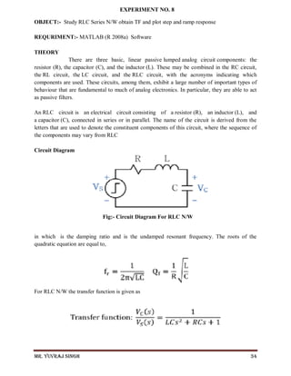
1. Ramp Response For RLC N/W
PROGRAM
R=37
L=.1
C=.1
W=sqrt(1/(L*C))
d=(R*sqrt(C/L))/2
N=[W*W]
D=[1,2*d*W,W*W]
T=tf(N,D)
A=0:0.001:50;
U=A;
lsim(T,U,A)
Title ('ramp responce for RLC N/W')
OUTPUT
R = 37
L = 0.1000
C = 0.1000
W = 10
d = 18.5000
N = 100
D = 1 370 100
Transfer function: 100
--------------------
s^2 + 370 s + 100

36. Mr. Yuvraj Singh 36
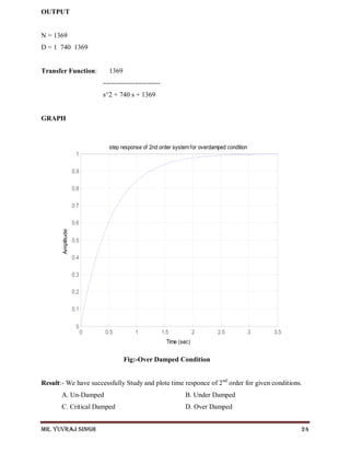
GRAPH
Fig:- Ramp Response For RLC N/W
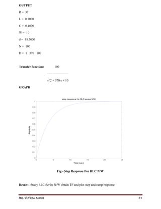
2. Step Response For RLC N/W
PROGRAM
R=37
L=.1
C=.1
W=sqrt(1/(L*C))
d=(R*sqrt(C/L))/2
N=[W*W]
D=[1,2*d*W,W*W]
T=tf(N,D)
step (T)
Title ('step responce for RLC series N/W')
ramp responce for RLC N/W
Time (sec)
Amplitude
0 5 10 15 20 25 30 35 40 45 50
0
5
10
15
20
25
30
35
40
45
50
System: T
Time (sec): 37
Amplitude: 33.3

37. Mr. Yuvraj Singh 37
OUTPUT
R = 37
L = 0.1000
C = 0.1000
W = 10
d = 18.5000
N = 100
D = 1 370 100
Transfer function: 100
--------------------
s^2 + 370 s + 10
GRAPH
Fig:- Step Response For RLC N/W
Result:- Study RLC Series N/W obtain TF and plot step and ramp response
0 5 10 15 20 25
0
0.1
0.2
0.3
0.4
0.5
0.6
0.7
0.8
0.9
1
step responce for RLC series N/W
Time (sec)
Amplitude