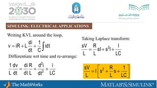
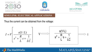
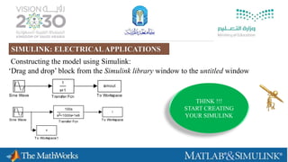
This document provides information about a MATLAB workshop for engineers. The workshop will cover basics of MATLAB/GUI/Simulink including how to solve simple problems and explore their capabilities. It will introduce MATLAB/GUI and Simulink through examples and topics like built-in functions, vectors/matrices, plotting, animation and functions. Specific modeling examples for mechanical and electrical applications using Simulink will also be presented. Participants will learn how to construct their own models in Simulink and display results.

1. MATLAB FOR ALL ENGINEERS
ADVANCED WORKSHOP
December-13th-2016
MECHANICAL ENGINEERING DEPARTMENT
Dr. SAEED J. ALMALOWI
COLLEGE OF ENGINEERING

2. What can you gain from the WORKSHOP ?
Know basics of MATLAB/GUI/Simulink?
know how to solve simple problems?
Know what MATLAB/GUI/Simulink is?
Know how to get started with MATLAB/GUI/Simulink?
Be able to explore MATLAB/GUI & Simulink on your own !
INTRODUCTION TO MATLAB/GUI&SIMULINK

3. 3
Built in functions
Getting Started
Vectors and Matrices
1. INTRODUCTION
2. GRAPHICAL USER INTERFACE
Examples
Introduction to MATLAB
GUI
M–files : script, Plots, Animation, and Functions 3. SIMULINK
Modeling Examples Simulink
CONTENTS

4.  Plots: 1D plot “ plot(t,x)”, 2D plot, “contourf(Z)’’ ,Surf plot , and 3D plot.
 Animation: gif (animated plots) or avi (Video).
 Functions:
The functions AVI ang GIF are interchangeable. They both turn all image files from a
given folder into a movie file.
function y = average(x)
if ~isvector(x) error('Input must be a vector')
end y = sum(x)/length(x);
end
PLOTS, ANIMATION, & FUNCTIONS

5. clear all
clc
x=0:0.01:1;
y1=-x.^3+x.^2+1;
y2=1./x.^2+10*x+5;
y3=x.^4+exp(-x)+2;
subplot(3,1,1)
plot(x,y1)
xlabel('x');ylabel('y1')
grid on
plot(x,y1)
subplot(3,1,2)
plot(x,y2)
xlabel('x');ylabel('y2')
grid on
subplot(3,1,3)
plot(x,y3)
xlabel('x');ylabel('y3')
grid on
SUBPLOTS
𝑦1 = −𝑥3
+ 𝑥2
+ 1
𝑦2 =
1
𝑥2 + 10𝑥 + 5
𝑦3 = 𝑥4
+ exp(−𝑥) + 2

6. frame = getframe(1);
im = frame2im(frame);
[imind,cm] = rgb2ind(im,256);
if k == 1;
imwrite(imind,cm,filename,'gif',
'Loopcount',inf);
else
imwrite(imind,cm,filename,'gif','WriteMode'
,'append');
end
filename = 'upwind.gif'; Open file and
name it!!!
Creating A
frame
Upwind Method (Scheme)
GIF ANIMATED PLOTS

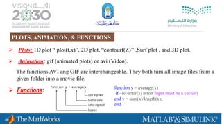
7. % Clear workspace
clear
clc
clf
% Define variables
N=100; % number of nodes
L=1; % The length of the domain
dx=L/(N);
x=0:dx:L;
ti=0; % Initial time
tf=0.8; % Final time
v=0.5; % Velcoity
dt=dx/v;
% Set Initial condition
uo=exp(-200*(x-0.25).^2);
u=uo;
unp1=uo;
% Loop through the time
nsteps=tf/dt;
t=ti;
filename = 'upwind.gif';
for k=1:nsteps
% BCs
u(1)=u(1);
u(N)=u(N);
% Exact Solution
% Calculate the FOU scheme
for i=2:N-1
unp1(i)=u(i)-v*dt/dx*(u(i)-u(i-1));
end
ua=exp(-200*(x-0.25-v*t).^2);
% Update u and t
t=t+dt;
u=unp1;
% Plot solution
plot(x,u,'bo-',x,ua,'r--')
xlabel('x')
ylabel('u')
shg
axis([ 0 L -0.5 1.5]);
grid on
pause (dt)
title(['Velcoity u (Time in [sec] is
' num2str(t) ')']);
drawnow
frame = getframe(1);
im = frame2im(frame);
[imind,cm] = rgb2ind(im,256);
if k == 1;
imwrite(imind,cm,filename,'gif',
'Loopcount',inf);
else
imwrite(imind,cm,filename,'gif','WriteM
ode','append');
end
end

8. To get GUI, write guide in command window as:

9. 𝑑𝑥2
𝑑𝑡2
+ 3η
𝑑𝑥
𝑑𝑡
+ 4𝑥 = 1
textbox1
function textbox1_Callback(hObject, eventdata,
handles)
% hObject handle to textbox1 (see GCBO)
% eventdata reserved - to be defined in a
future version of MATLAB
% handles structure with handles and user
data (see GUIDATA)
% Hints: get(hObject,'String') returns contents
of textbox1 as text
% str2double(get(hObject,'String'))
returns contents of textbox1 as a double
str=get(hObject,'String');
set(handles.slider1,'value',str2num(str));

10. 𝑑𝑥2
𝑑𝑡2
+ 3η
𝑑𝑥
𝑑𝑡
+ 4𝑥 = 1
function slider1_Callback(hObject, eventdata,
handles)
% hObject handle to slider1 (see GCBO)
% eventdata reserved - to be defined in a future
version of MATLAB
% handles structure with handles and user data
(see GUIDATA)
% Hints: get(hObject,'Value') returns position of
slider
% get(hObject,'Min') and
get(hObject,'Max') to determine range of slider
val=get(hObject,'Value');
set(handles.textbox1,'String',num2str(val));
slider1

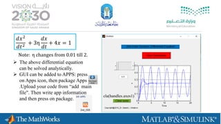
11. 𝑑𝑥2
𝑑𝑡2
+ 3η
𝑑𝑥
𝑑𝑡
+ 4𝑥 = 1
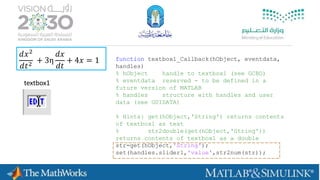
function runsimulation_Callback(hObject, eventdata, handles)
% hObject handle to runsimulation (see GCBO)
% eventdata reserved - to be defined in a future version of
MATLAB
% handles structure with handles and user data (see
GUIDATA)
eta=get(handles.slider1,'value');
G=tf(1,[1,3*eta,4])
time=linspace(0,20,200);
[x]=step(G,time);
axes(handles.axes1);
plot(time,x)
hold on
grid on
xlabel('Time')
ylabel('x')

12. cla(handles.axes1)
𝑑𝑥2
𝑑𝑡2
+ 3η
𝑑𝑥
𝑑𝑡
+ 4𝑥 = 1
Note: η changes from 0.01 till 2.
 The above differential equation
can be solved analytically.
 GUI can be added to APPS: press
on Apps icon, then package Apps
.Upload your code from “add main
file". Then write app information
and then press on package.

13. 13
Model – simplified representation of a system – e.g. using mathematical
equation.
We simulate a model to study the behavior of a system – need to
verify that our model is correct – expect results
Knowing how to use Simulink or MATLAB does not mean that you know how to model a
system.
SIMULINK: WHY DO WE NEED IT?!!

14. Start Simulink by typing simulink at Matlab prompt
Simulink library and untitled windows appear
It is here where we
construct our model.
It is where we
obtain the blocks to
construct our model
SIMULINK: LIBRARY

15.  Creating a New Model
 Press on New, then Model.
 Save as your model.
 Go to Simulink library browse
to add an element.

16. SIMULINK: ELECTRICAL APPLICATIONS
SCOPE/ RESULTS

17. ma = F t − kx − bv
Second Order Dynamic System
MECHANICALAPPLICATIONS

18. SIMULINK: ELECTRICALAPPLICATIONS
Simple Circuit- Krishof's Voltage and Current Law.

19. Problem: We need to simulate the resonant circuit and display the current waveform as we
change the frequency dynamically.
i 10  100 uF
0.01
H
Varies 
from 0 to
2000 rad/s
Observe the current. What do we expect ?
The amplitude of the current waveform will become maximum at resonant frequency, i.e. at
 = 1000 rad/s
+
v(t) = 5 sin t
–
SIMULINK: ELECTRICALAPPLICATIONS

20.  idt
C
1
dt
di
LiRv
Writing KVL around the loop,
LC
i
dt
id
L
R
dt
di
dt
dv
L
1
2
2

Differentiate wrt time and re-arrange:
Taking Laplace transform:
LC
I
IssI
L
R
L
sV 2






LC
1
s
L
R
sI
L
sV 2
SIMULINK: ELECTRICALAPPLICATIONS

21. Thus the current can be obtained from the voltage:












LC
s
L
R
s
Ls
VI
1
)/1(
2
LC
1
s
L
R
s
)L/1(s
2

V I
SIMULINK: ELECTRICALAPPLICATIONS

22. Constructing the model using Simulink:
1
s+1
Transfer Fcn
simout
To WorkspaceSine Wave
‘Drag and drop’ block from the Simulink library window to the untitled window
100s
s +1000s+1e62
Transfer Fcn
v
To Workspace1
i
To WorkspaceSine Wave
THINK !!!
START CREATING
YOUR SIMULINK
SIMULINK: ELECTRICALAPPLICATIONS

23. talent@taibahu.edu.sa
Contact us
@talent_taibah
QUESTIONS??????