Thank you for the overview of Simulink. Let me know if you need any other information.

1. MIT OpenCourseWare
http://ocw.mit.edu
6.094 Introduction to MATLAB®
January (IAP) 2009
For information about citing these materials or our Terms of Use, visit: http://ocw.mit.edu/terms.

2. 6.094
Introduction to Programming in MATLAB®
Lecture 5: Simulink®
Sourav Dey
Danilo Šćepanović
Ankit Patel
Patrick Ho
IAP 2009

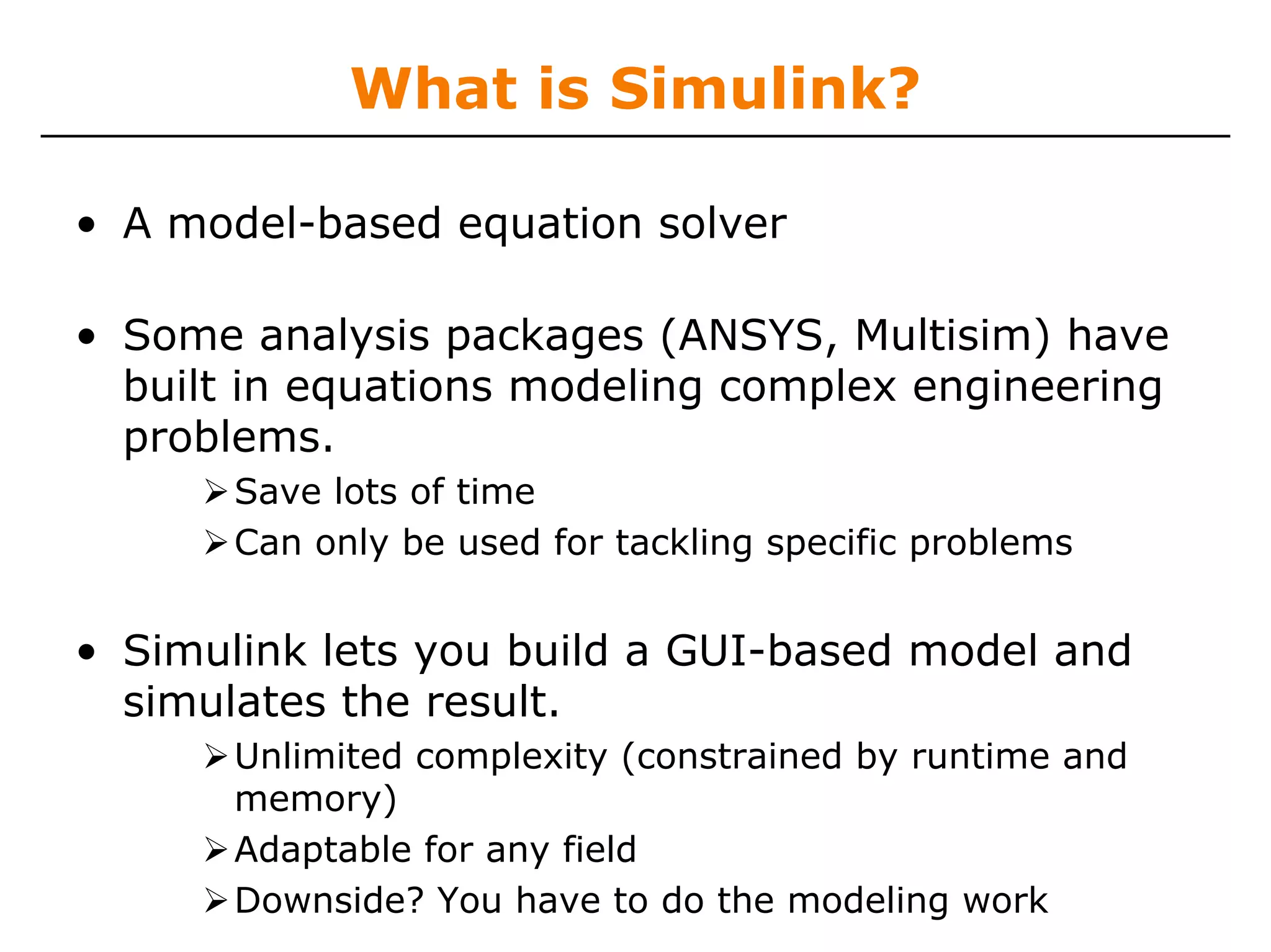
3. What is Simulink?
• A model-based equation solver
• Some analysis packages (ANSYS, Multisim) have
built in equations modeling complex engineering
problems.
Save lots of time
Can only be used for tackling specific problems
• Simulink lets you build a GUI-based model and
simulates the result.
Unlimited complexity (constrained by runtime and
memory)
Adaptable for any field
Downside? You have to do the modeling work

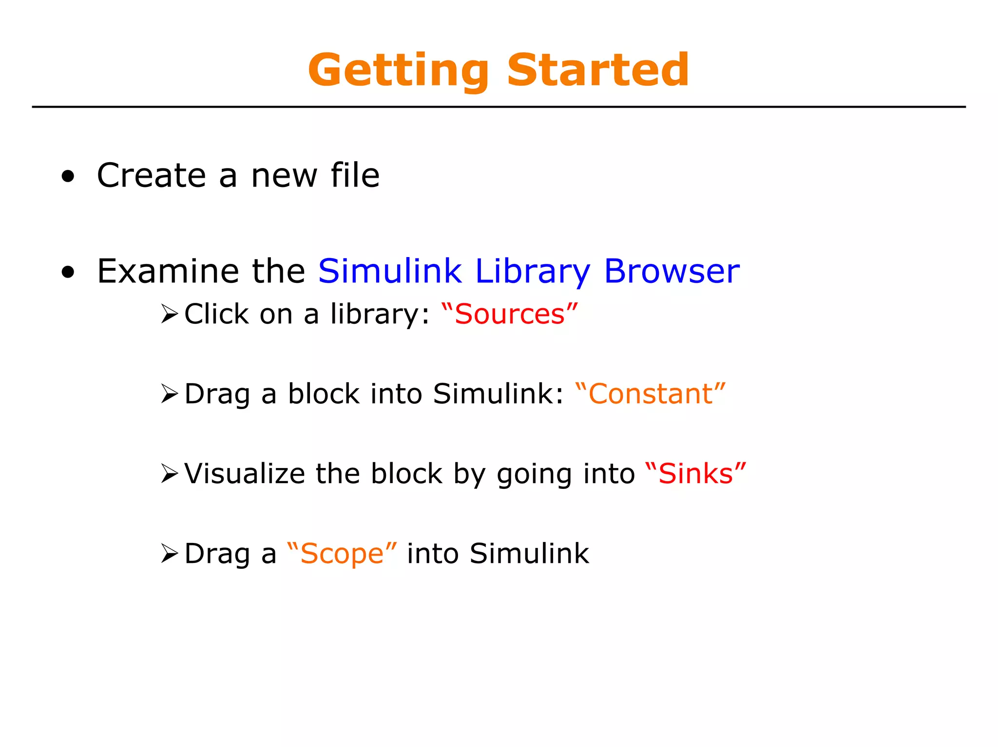
4. Getting Started
• Create a new file
• Examine the Simulink Library Browser
Click on a library: “Sources”
Drag a block into Simulink: “Constant”
Visualize the block by going into “Sinks”
Drag a “Scope” into Simulink

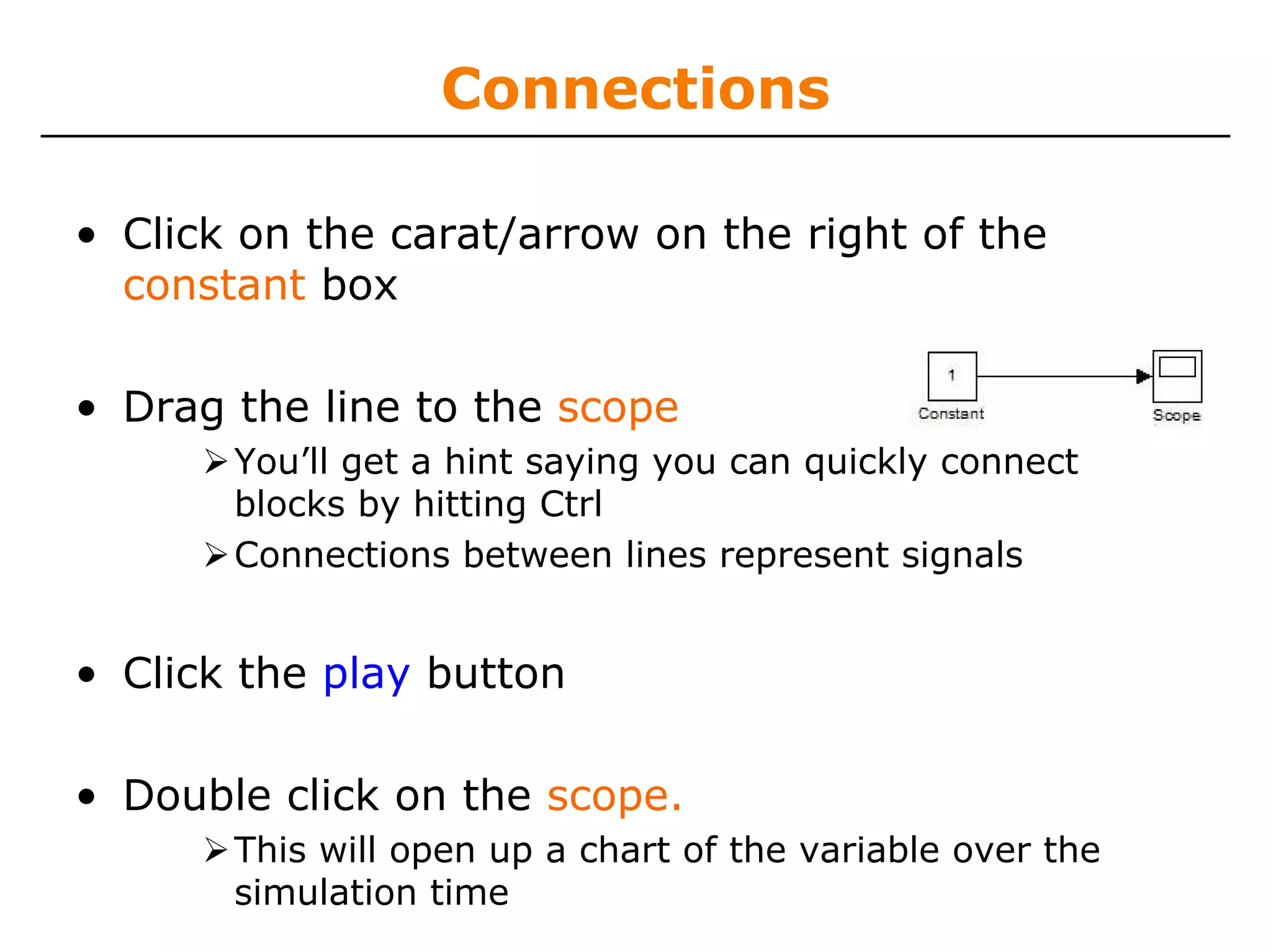
5. Connections
• Click on the carat/arrow on the right of the
constant box
• Drag the line to the scope
You’ll get a hint saying you can quickly connect
blocks by hitting Ctrl
Connections between lines represent signals
• Click the play button
• Double click on the scope.
This will open up a chart of the variable over the
simulation time

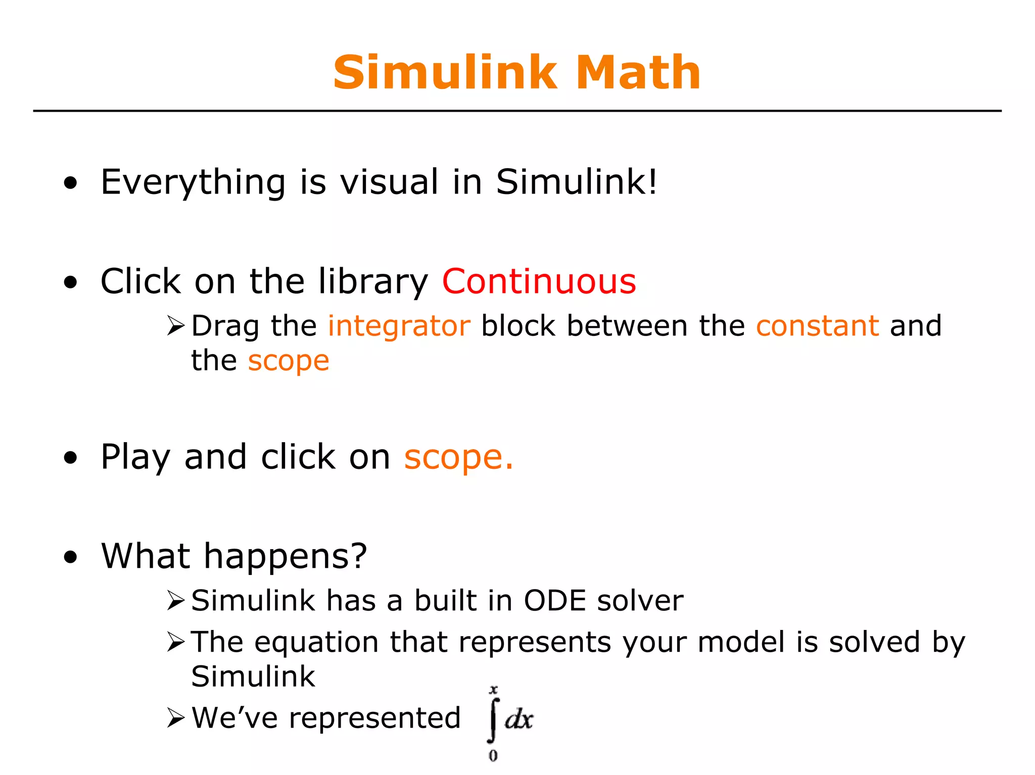
6. Simulink Math
• Everything is visual in Simulink!
• Click on the library Continuous
Drag the integrator block between the constant and
the scope
• Play and click on scope.
• What happens?
Simulink has a built in ODE solver
The equation that represents your model is solved by
Simulink
We’ve represented

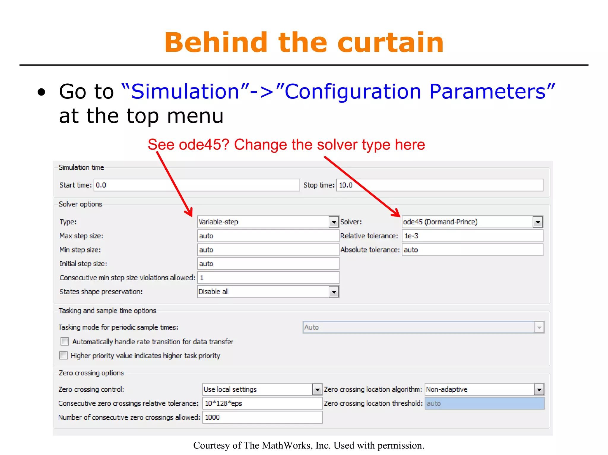
7. Behind the curtain
• Go to “Simulation”->”Configuration Parameters”
at the top menu
See ode45? Change the solver type here
Courtesy of The MathWorks, Inc. Used with permission.

8. So what’s going on?
• The toolboxes Simulink provides you are full of
modeling tools
• By selecting components that correspond to your
model, you can design a simulation

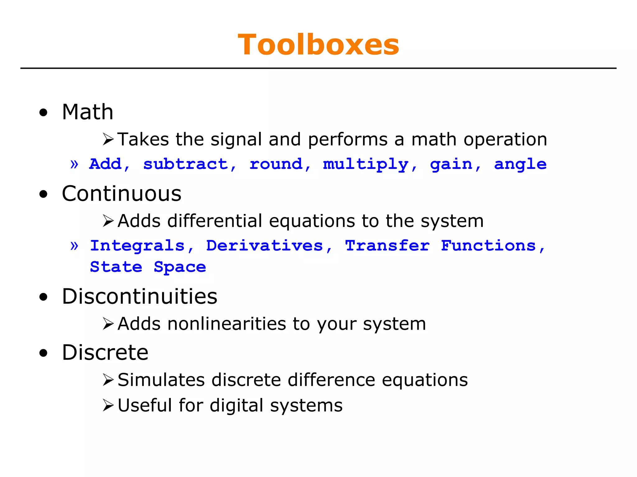
9. Toolboxes
• Math
Takes the signal and performs a math operation
» Add, subtract, round, multiply, gain, angle
• Continuous
Adds differential equations to the system
» Integrals, Derivatives, Transfer Functions,
State Space
• Discontinuities
Adds nonlinearities to your system
• Discrete
Simulates discrete difference equations
Useful for digital systems

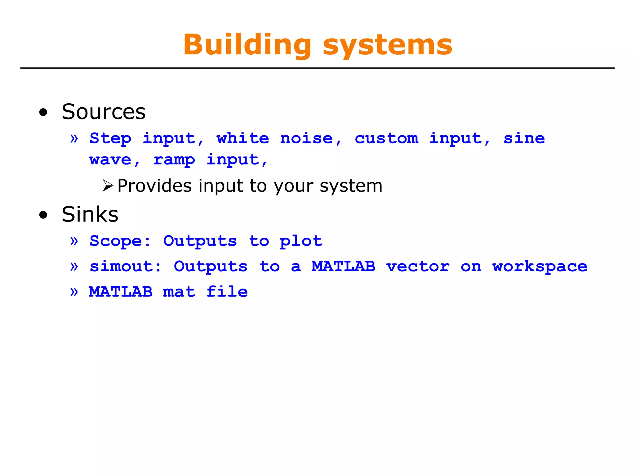
10. Building systems
• Sources
» Step input, white noise, custom input, sine
wave, ramp input,
Provides input to your system
• Sinks
» Scope: Outputs to plot
» simout: Outputs to a MATLAB vector on workspace
» MATLAB mat file

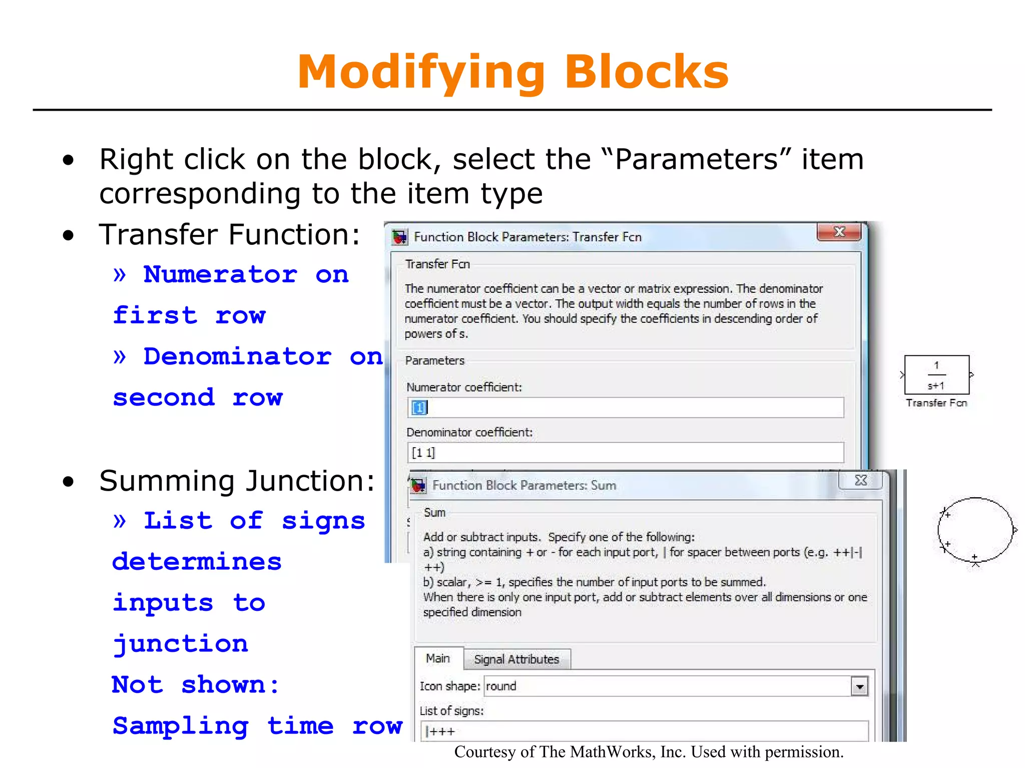
11. Modifying Blocks
• Right click on the block, select the “Parameters” item
corresponding to the item type
• Transfer Function:
» Numerator on
first row
» Denominator on
second row
• Summing Junction:
» List of signs
determines
inputs to
junction
Not shown:
Sampling time row
Courtesy of The MathWorks, Inc. Used with permission.

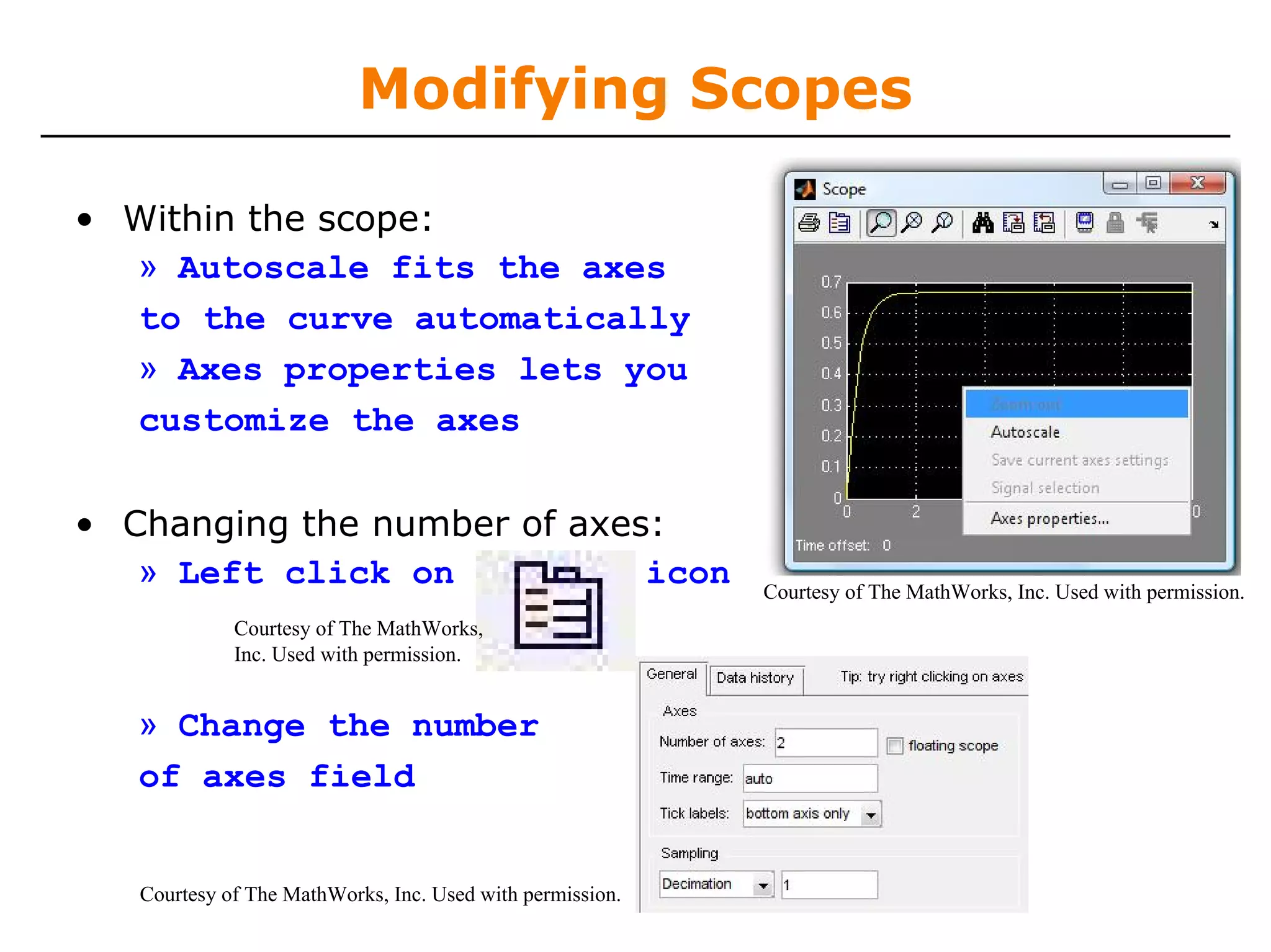
12. Modifying Scopes
• Within the scope:
» Autoscale fits the axes
to the curve automatically
» Axes properties lets you
customize the axes
• Changing the number of axes:
» Left click on icon Courtesy of The MathWorks, Inc. Used with permission.
Courtesy of The MathWorks,
Inc. Used with permission.
» Change the number
of axes field
Courtesy of The MathWorks, Inc. Used with permission.

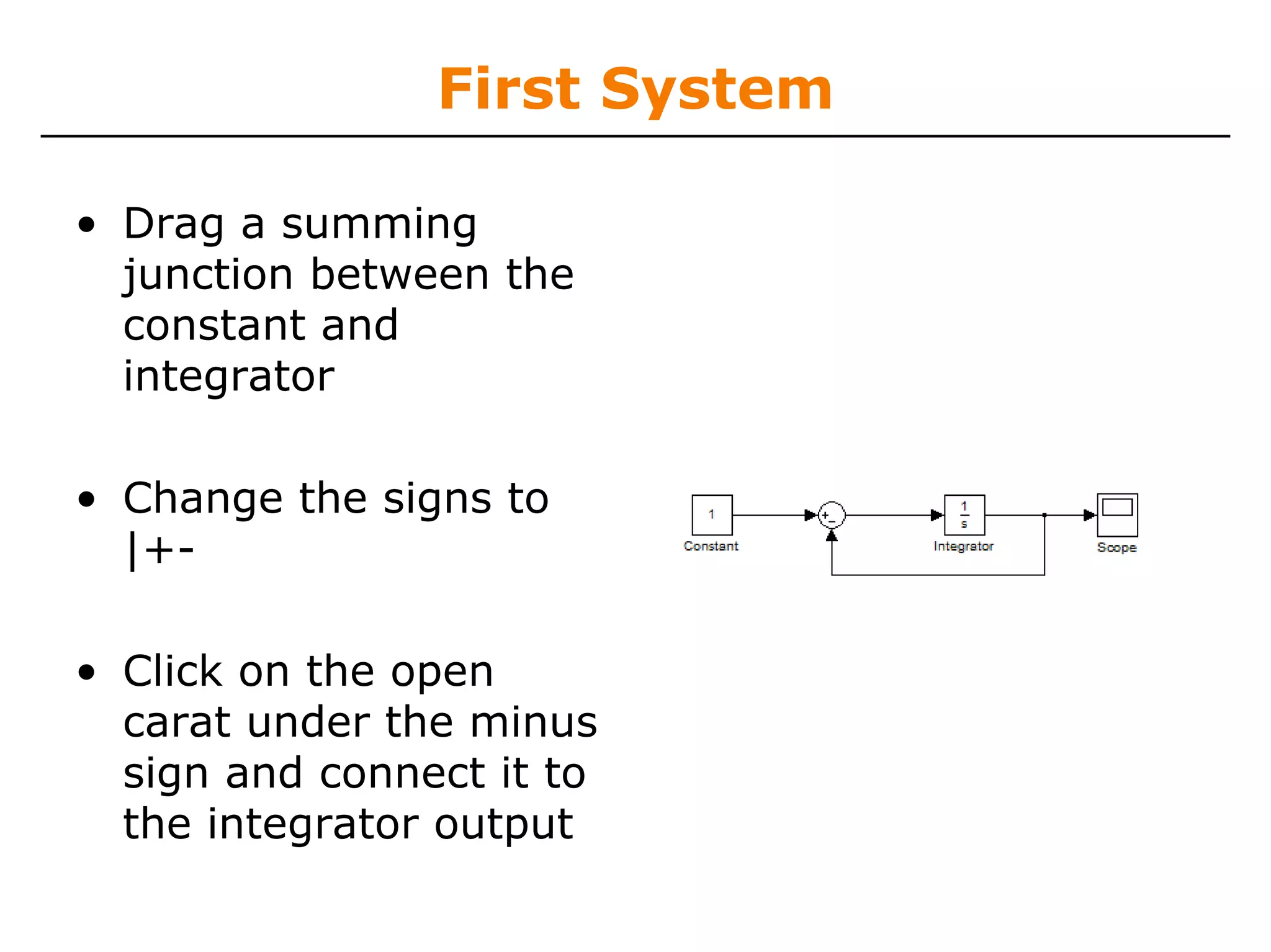
13. First System
• Drag a summing
junction between the
constant and
integrator
• Change the signs to
|+-
• Click on the open
carat under the minus
sign and connect it to
the integrator output

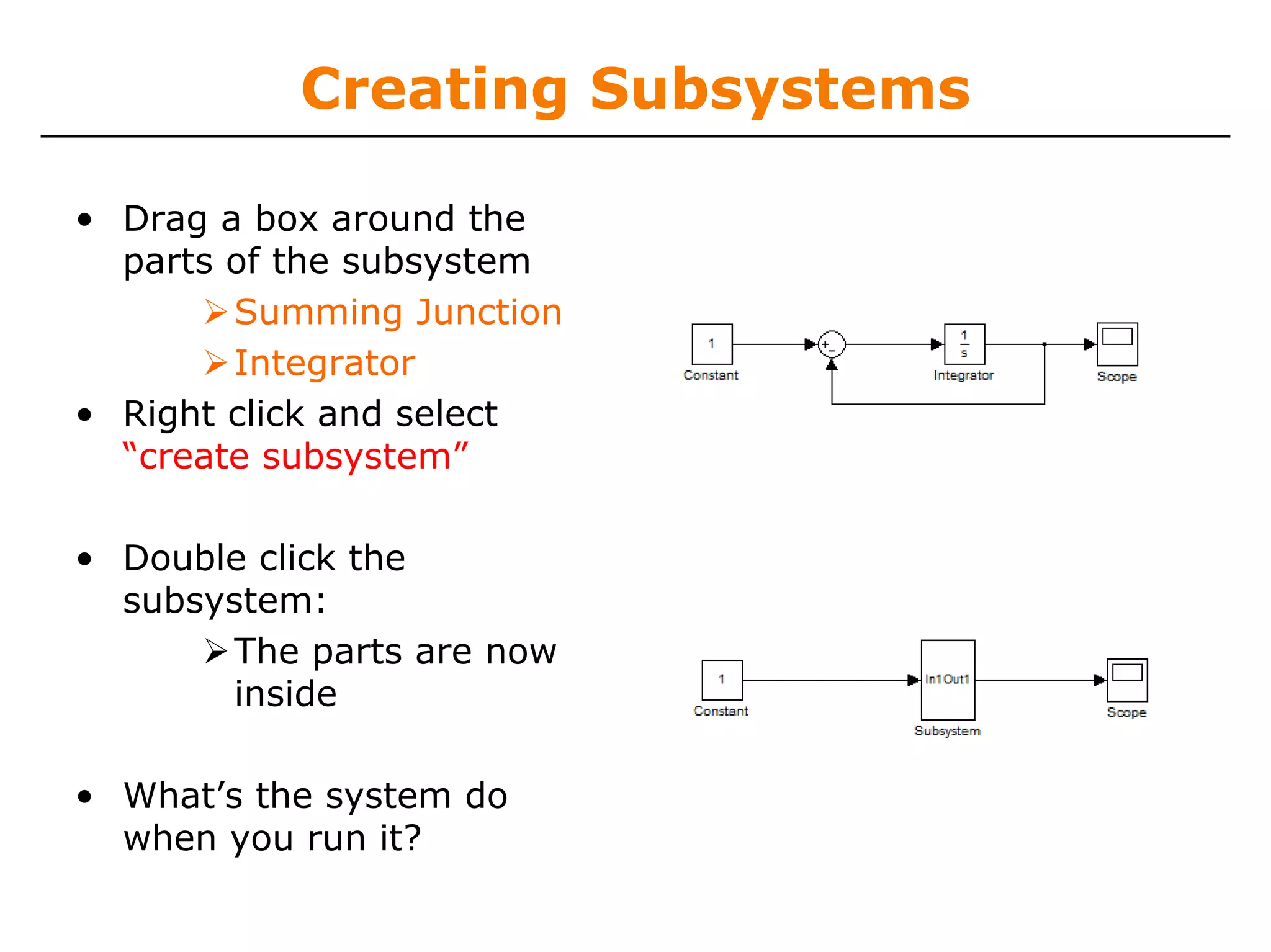
14. Creating Subsystems
• Drag a box around the
parts of the subsystem
Summing Junction
Integrator
• Right click and select
“create subsystem”
• Double click the
subsystem:
The parts are now
inside
• What’s the system do
when you run it?

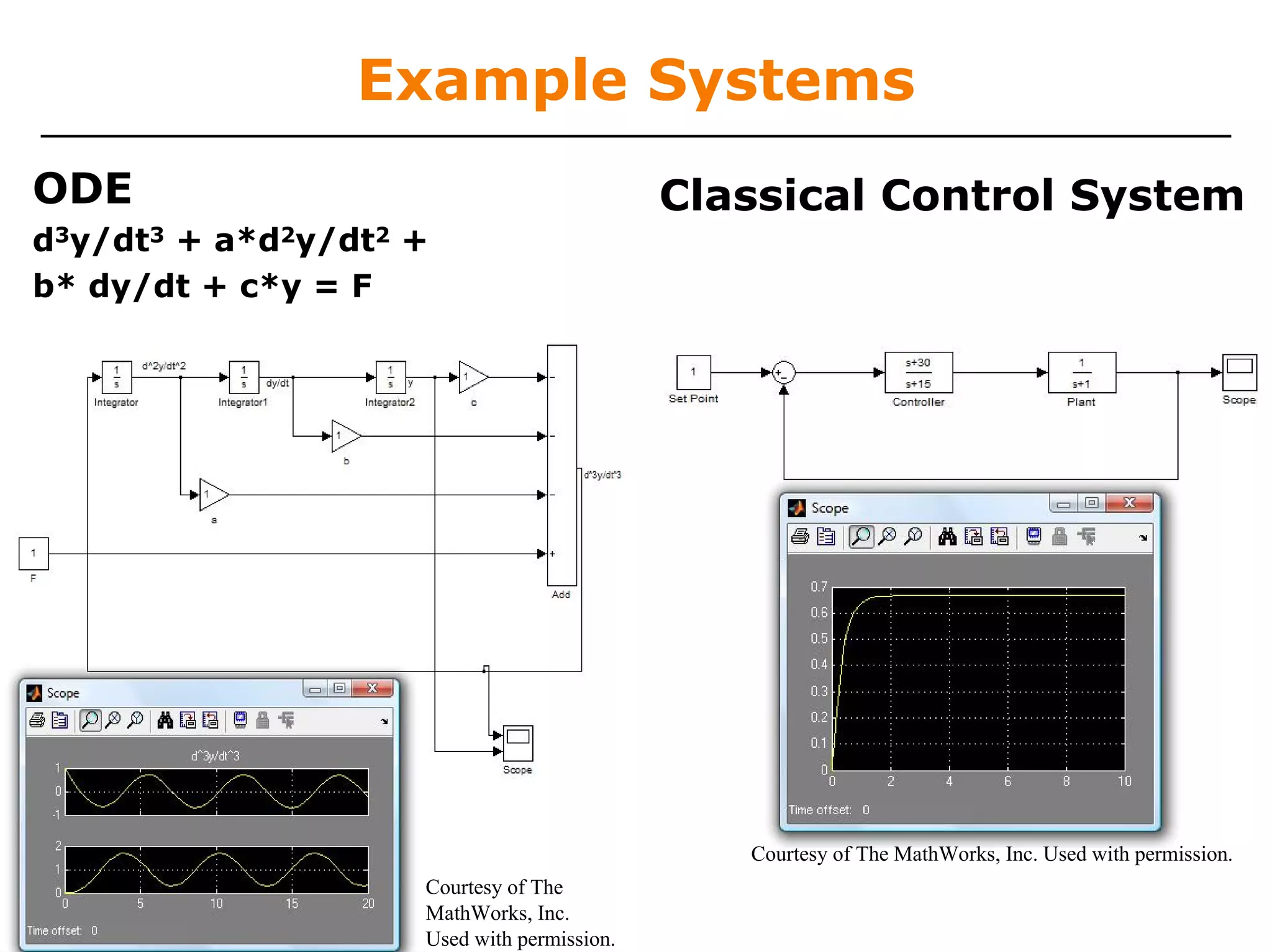
15. Example Systems
ODE Classical Control System
d3y/dt3 + a*d2y/dt2 +
b* dy/dt + c*y = F
Courtesy of The MathWorks, Inc. Used with permission.
Courtesy of The
MathWorks, Inc.
Used with permission.

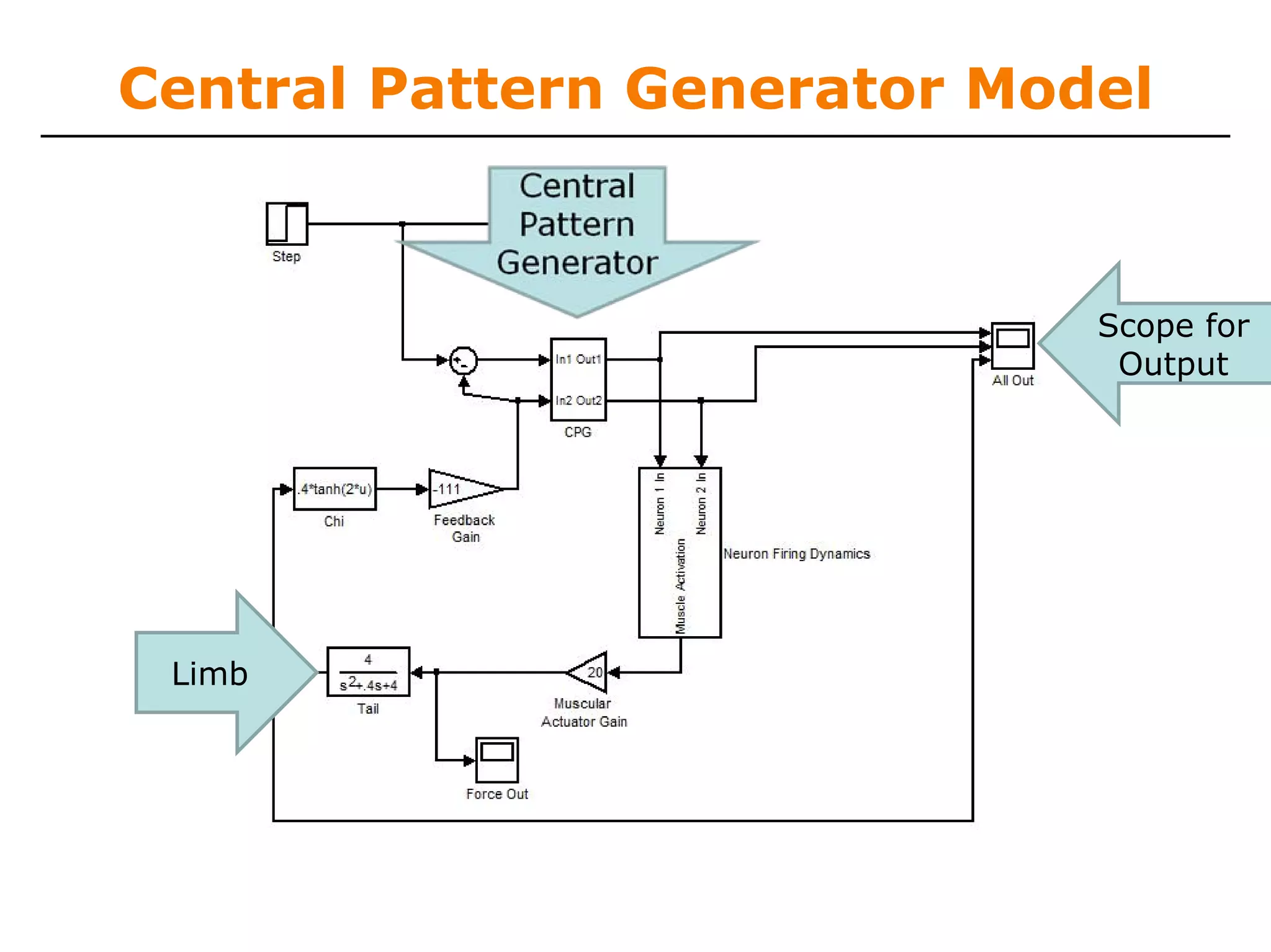
16. Example: Nervous System
• Neural circuits in animals often exhibit oscillatory behavior
• Use Simulink to model one behavior of this type:
Locomotion
– Limbs go “Left-right, left-right, left-right”
• Locomotive behaviors are generated by “central pattern
generators,” which oscillate on their own naturally
• When connected to an appendage, the central pattern
generator will adapt its frequency and move the
appendage. Open “RIOCPGDemo.mdl”
• Model based on Iwasaki, T., Zheng, M. (2006a). Sensory feedback
mechanism underlying entrainment of central pattern generator to
mechanical resonance. Biological Cybernetics, 94(4), 245-261

17. Central Pattern Generator Model
Scope for
Output
Limb

18. Playing with the model
• Look at scopes
What are the output signals?
• Delete signals
Especially the signal after the feedback gain
• Change gains
Muscular actuator gains
Switch feedback gain from negative to positive
• Look inside subsystems
What’s inside the CPG?
What’s inside the neuron firing dynamics?

19. Toolboxes
• Simulink has many advanced toolboxes
Control Systems
Neural Networks
Signal Processing
SimMechanics
Virtual Reality
Real Time
• Hopefully you’ll get to use some of these powerful tools!