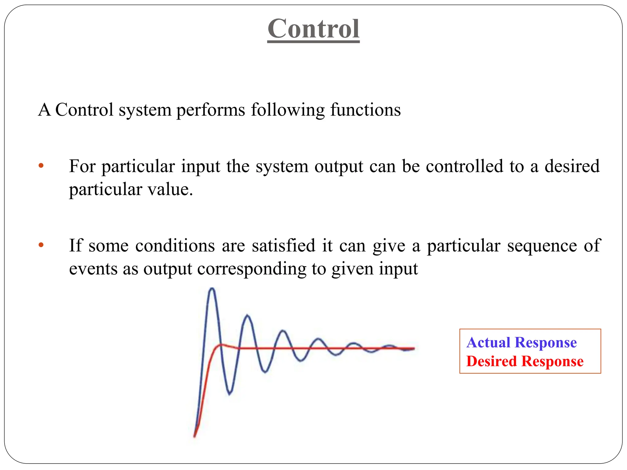
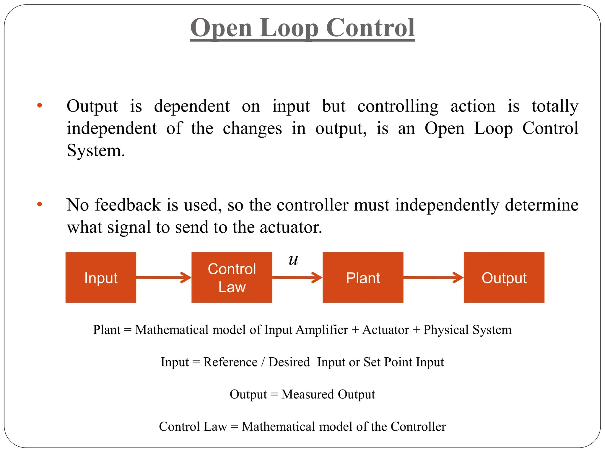
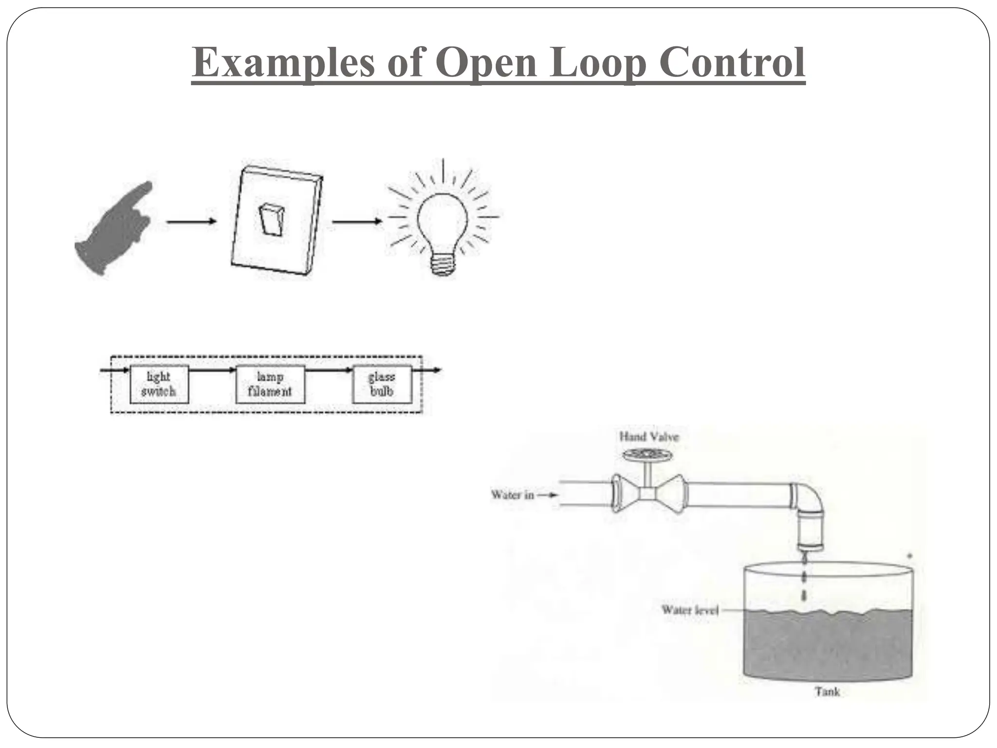
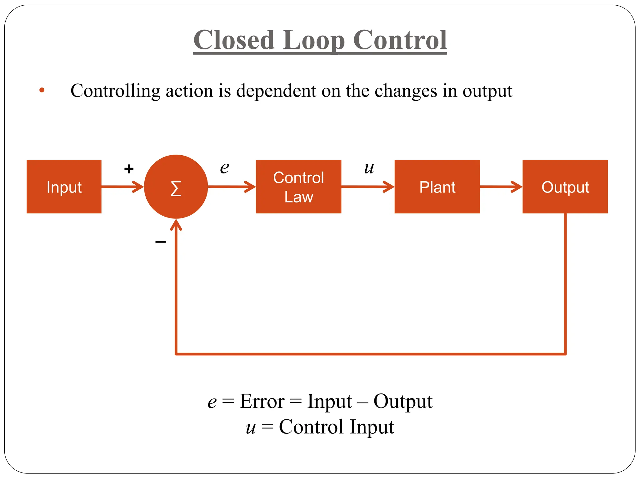
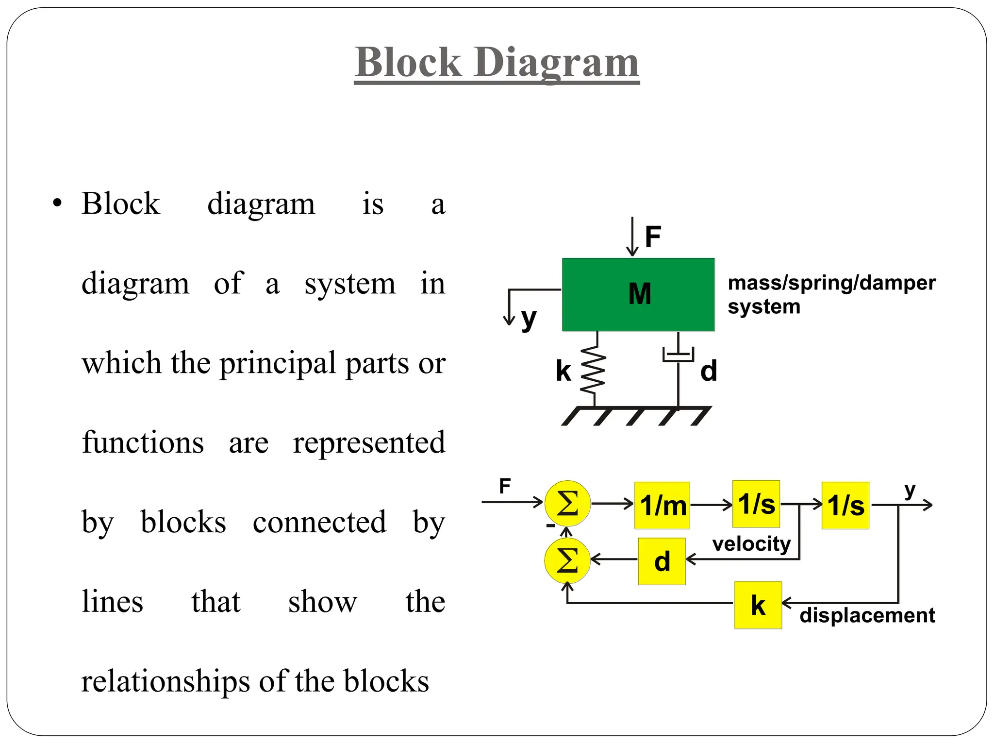
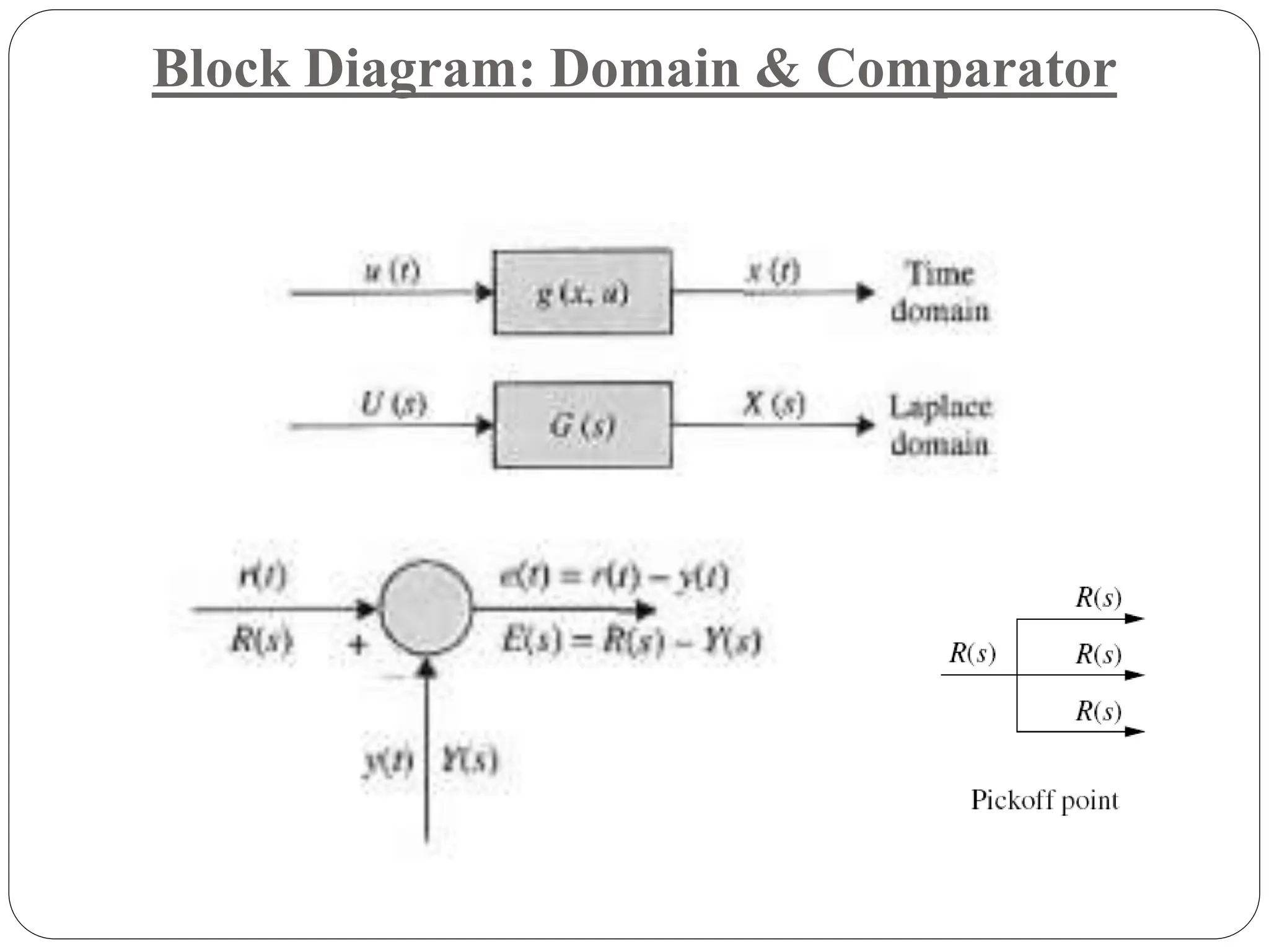
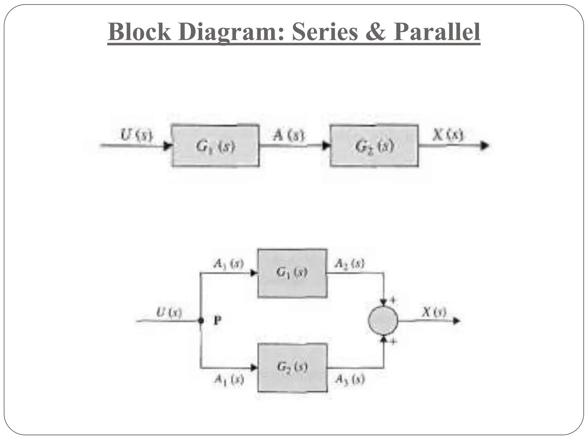
Lecture Notes / PPT
UNIT II
Mechatronics – 302050
Syllabus
Block Diagram Representation
 Open and Closed loop control system,
 Identification of key elements of mechatronics systems and
represent into block diagram (Electro-Mechanical Systems),
 Concept of transfer function,
 Block diagram reduction principles,
 Applications of mechatronics systems:- Household, Automotive,
Shop floor, Industrial.
Objectives
1. Understand key elements of Mechatronics system,
representation into block diagram
2. Understand concept of transfer function, reduction and analysis
3. Understand principles of sensors, its characteristics, interfacing
with DAQ microcontroller
4. Understand the concept of PLC system and its ladder
programming, and significance of PLC systems in industrial
application
5. Understand the system modeling and analysis in time domain
and frequency domain.
6. Understand control actions such as Proportional, derivative and
integral and study its significance in industrial applications.
Outcomes
1. Identification of key elements of mechatronics system and its
representation in terms of block diagram
2. Understanding the concept of signal processing and use of
interfacing systems such as ADC, DAC, digital I/O
3. Interfacing of Sensors, Actuators using appropriate DAQ
micro-controller
4. Time and Frequency domain analysis of system model (for
control application)
5. PID control implementation on real time systems
6. Development of PLC ladder programming and implementation
of real life system
Assumed Knowledge
Dynamics:
 Engineering Mechanics
Mathematics
 Engineering Mathematics (I, II & III)
Reference Books
 Alciatore & Histand, Introduction to Mechatronics and
Measurement system, 4th Edition, McGraw Hill publication,
2011
 Golnaraghi & Kuo, Automatic Control Systems, John Wiley
publications, 2010
Control
A Control system performs following functions
• For particular input the system output can be controlled to a desired
particular value.
• If some conditions are satisfied it can give a particular sequence of
events as output corresponding to given input
Actual Response
Desired Response
Controllability
(Out of Syllabus)
 Before a controller is implemented it is necessary to test the
“Controllability” of the system
 Controllability is the ability of the system, to be controlled /
provide desired performance, provided an external disturbance
is available.
Open Loop Control
• Output is dependent on input but controlling action is totally
independent of the changes in output, is an Open Loop Control
System.
• No feedback is used, so the controller must independently determine
what signal to send to the actuator.
Input
Control
Law
Plant Output
u
Plant = Mathematical model of Input Amplifier + Actuator + Physical System
Input = Reference / Desired Input or Set Point Input
Output = Measured Output
Control Law = Mathematical model of the Controller
Examples of Open Loop Control
Advantages and Dis-advantages of Open Loop
Control
Advantages:
 Simple in construction
 Low cost
 Convenient to implement when output is difficult to measure
Disadvantages:
 The controller never actually knows if the actuator did what it
was supposed to do, i.e. it is inaccurate
 Unable to sense the environmental changes or disturbances
Closed Loop Control
e = Error = Input – Output
u = Control Input
Input
Control
Law
Plant Output
∑
+
_
e u
• Controlling action is dependent on the changes in output
Examples of Closed Loop Control
Examples of Automatic Closed Loop Control
Advantages:
 Accurate, since the controller modifies and manipulates the
actuating signal such that the error in the system will be zero.
 Self-correcting
 Senses the environmental changes, and disturbances in the
system.
Disadvantages:
 Complicated to design
 Costly
 Instable, since due to feedback , system tries to correct the error.
Advantages and Dis-advantages of Closed Loop Control
Key Elements in Mechatronic System
Key Elements in Mechatronic System: Example of Electro-
Mechanical System
Response of System
0 5 10 15 20 25 30 35 40 45 50
time (sec)
0 5 10 15 20 25 30 35 40 45 50
time (sec)
0 5 10 15 20 25 30 35 40 45 50
time (sec)
time (sec)
0 5 10 15 20 25 30 35 40 45 50
time (sec)
0 5 10 15 20 25 30 35 40 45 50
Transfer Function Models
 Why TF?
 Because it is easier / better to assess some things
using classical techniques, such as gain and phase
margin.
 How to determine TF?
 Derive the Governing Differential Equation
 Assume I.C=Zero and
 Take Laplace transform of output
 Take Laplace transform of input
 Transfer function = L (output) / L (input)
1/s 1/s
1/m
M
F
y
k d
mass/spring/dam
system
F
Translational Mechanical Example 1
       
 
  k
ds
ms
s
f
s
y
s
f
s
ky
s
dsy
s
y
ms
f
ky
y
d
y
m













2
2
1
Input
Output
T.F
sides
both
of
Laplace
taking
and
0
I.C
Assuming
(EOM)
motion
of
Equation 


Translational Mechanical Example 1
Block Diagram
• Block diagram is a
diagram of a system in
which the principal parts or
functions are represented
by blocks connected by
lines that show the
relationships of the blocks
1/s 1/s
d
k
1/m
M
F
y
k d
mass/spring/damper
system
F y
displacement
velocity
Block Diagram
 Comparator
 Input/Reference/Output/Disturb
ance / Feedback Signal
 Blocks to represent:
 Sensor, Actuator, Plant,
Controller, Amplifier etc (in
symbolic form / transfer
function form)
 Subsystem is represented as a
block with an input, an output,
and a transfer function
 When multiple subsystems are
interconnected, a few more
schematic elements must be
added to the block diagram
 These new elements are
summing junctions and pickoff
points.
Block Diagram: Domain & Comparator
Block Diagram: Series & Parallel
Block Diagram: Feedback
 
 
 
   
 
 
 
   
s
H
s
G
s
G
s
R
s
Y
s
H
s
G
s
G
s
R
s
Y






1
TF
loop
Closed
1
TF
loop
Closed
Reduction techniques
2
G
1
G 2
1G
G
2. Moving a summing point behind a block
G G
G
1
G
2
G
2
1 G
G 
1. Combining blocks in cascade or in parallel
5. Moving a pickoff point ahead of a block
G G
G G
G
1
G
3. Moving a summing point ahead of a block
G G
G
1
4. Moving a pickoff point behind a block
6. Eliminating a feedback loop
G
H
GH
G

1
7. Swap with two neighboring summing points
A B A
B
G
1

H
G
G

1
Moving Blocks to Create Familiar Forms
Example 1
Example 1
Example 2
Example 2
Example 3
Example 3
Example 4
Example 5
Example 5
Example 5
Example 5
Applications of Mechatronic System
• Household
• Refrigerator
• Washing m/c
• Microwave
• Automotive
• Fuel injection system
• Power steering
• Air conditioner
• Shop floor
• Tool monitoring system
• Automated guided vehicle
• Conveyor system
• Bottle filing plant.
Fuel Injection
Electric Power Steering

Mechatrnoics PPT Lecture notes on Actuators

  • 1.
    Lecture Notes /PPT UNIT II Mechatronics – 302050
  • 2.
    Syllabus Block Diagram Representation Open and Closed loop control system,  Identification of key elements of mechatronics systems and represent into block diagram (Electro-Mechanical Systems),  Concept of transfer function,  Block diagram reduction principles,  Applications of mechatronics systems:- Household, Automotive, Shop floor, Industrial.
  • 3.
    Objectives 1. Understand keyelements of Mechatronics system, representation into block diagram 2. Understand concept of transfer function, reduction and analysis 3. Understand principles of sensors, its characteristics, interfacing with DAQ microcontroller 4. Understand the concept of PLC system and its ladder programming, and significance of PLC systems in industrial application 5. Understand the system modeling and analysis in time domain and frequency domain. 6. Understand control actions such as Proportional, derivative and integral and study its significance in industrial applications.
  • 4.
    Outcomes 1. Identification ofkey elements of mechatronics system and its representation in terms of block diagram 2. Understanding the concept of signal processing and use of interfacing systems such as ADC, DAC, digital I/O 3. Interfacing of Sensors, Actuators using appropriate DAQ micro-controller 4. Time and Frequency domain analysis of system model (for control application) 5. PID control implementation on real time systems 6. Development of PLC ladder programming and implementation of real life system
  • 5.
    Assumed Knowledge Dynamics:  EngineeringMechanics Mathematics  Engineering Mathematics (I, II & III)
  • 6.
    Reference Books  Alciatore& Histand, Introduction to Mechatronics and Measurement system, 4th Edition, McGraw Hill publication, 2011  Golnaraghi & Kuo, Automatic Control Systems, John Wiley publications, 2010
  • 7.
    Control A Control systemperforms following functions • For particular input the system output can be controlled to a desired particular value. • If some conditions are satisfied it can give a particular sequence of events as output corresponding to given input Actual Response Desired Response
  • 8.
    Controllability (Out of Syllabus) Before a controller is implemented it is necessary to test the “Controllability” of the system  Controllability is the ability of the system, to be controlled / provide desired performance, provided an external disturbance is available.
  • 9.
    Open Loop Control •Output is dependent on input but controlling action is totally independent of the changes in output, is an Open Loop Control System. • No feedback is used, so the controller must independently determine what signal to send to the actuator. Input Control Law Plant Output u Plant = Mathematical model of Input Amplifier + Actuator + Physical System Input = Reference / Desired Input or Set Point Input Output = Measured Output Control Law = Mathematical model of the Controller
  • 10.
    Examples of OpenLoop Control
  • 11.
    Advantages and Dis-advantagesof Open Loop Control Advantages:  Simple in construction  Low cost  Convenient to implement when output is difficult to measure Disadvantages:  The controller never actually knows if the actuator did what it was supposed to do, i.e. it is inaccurate  Unable to sense the environmental changes or disturbances
  • 12.
    Closed Loop Control e= Error = Input – Output u = Control Input Input Control Law Plant Output ∑ + _ e u • Controlling action is dependent on the changes in output
  • 13.
    Examples of ClosedLoop Control
  • 14.
    Examples of AutomaticClosed Loop Control
  • 15.
    Advantages:  Accurate, sincethe controller modifies and manipulates the actuating signal such that the error in the system will be zero.  Self-correcting  Senses the environmental changes, and disturbances in the system. Disadvantages:  Complicated to design  Costly  Instable, since due to feedback , system tries to correct the error. Advantages and Dis-advantages of Closed Loop Control
  • 16.
    Key Elements inMechatronic System
  • 17.
    Key Elements inMechatronic System: Example of Electro- Mechanical System
  • 18.
    Response of System 05 10 15 20 25 30 35 40 45 50 time (sec) 0 5 10 15 20 25 30 35 40 45 50 time (sec) 0 5 10 15 20 25 30 35 40 45 50 time (sec) time (sec) 0 5 10 15 20 25 30 35 40 45 50 time (sec) 0 5 10 15 20 25 30 35 40 45 50
  • 19.
    Transfer Function Models Why TF?  Because it is easier / better to assess some things using classical techniques, such as gain and phase margin.  How to determine TF?  Derive the Governing Differential Equation  Assume I.C=Zero and  Take Laplace transform of output  Take Laplace transform of input  Transfer function = L (output) / L (input)
  • 20.
  • 21.
               k ds ms s f s y s f s ky s dsy s y ms f ky y d y m              2 2 1 Input Output T.F sides both of Laplace taking and 0 I.C Assuming (EOM) motion of Equation    Translational Mechanical Example 1
  • 22.
    Block Diagram • Blockdiagram is a diagram of a system in which the principal parts or functions are represented by blocks connected by lines that show the relationships of the blocks 1/s 1/s d k 1/m M F y k d mass/spring/damper system F y displacement velocity
  • 23.
    Block Diagram  Comparator Input/Reference/Output/Disturb ance / Feedback Signal  Blocks to represent:  Sensor, Actuator, Plant, Controller, Amplifier etc (in symbolic form / transfer function form)  Subsystem is represented as a block with an input, an output, and a transfer function  When multiple subsystems are interconnected, a few more schematic elements must be added to the block diagram  These new elements are summing junctions and pickoff points.
  • 24.
  • 25.
  • 26.
    Block Diagram: Feedback                    s H s G s G s R s Y s H s G s G s R s Y       1 TF loop Closed 1 TF loop Closed
  • 27.
    Reduction techniques 2 G 1 G 2 1G G 2.Moving a summing point behind a block G G G 1 G 2 G 2 1 G G  1. Combining blocks in cascade or in parallel
  • 28.
    5. Moving apickoff point ahead of a block G G G G G 1 G 3. Moving a summing point ahead of a block G G G 1 4. Moving a pickoff point behind a block
  • 29.
    6. Eliminating afeedback loop G H GH G  1 7. Swap with two neighboring summing points A B A B G 1  H G G  1
  • 30.
    Moving Blocks toCreate Familiar Forms
  • 31.
    Moving Blocks toCreate Familiar Forms
  • 32.
  • 33.
  • 34.
  • 35.
  • 36.
  • 37.
  • 38.
  • 39.
  • 40.
  • 41.
  • 42.
  • 43.
    Applications of MechatronicSystem • Household • Refrigerator • Washing m/c • Microwave • Automotive • Fuel injection system • Power steering • Air conditioner • Shop floor • Tool monitoring system • Automated guided vehicle • Conveyor system • Bottle filing plant.
  • 44.
  • 45.