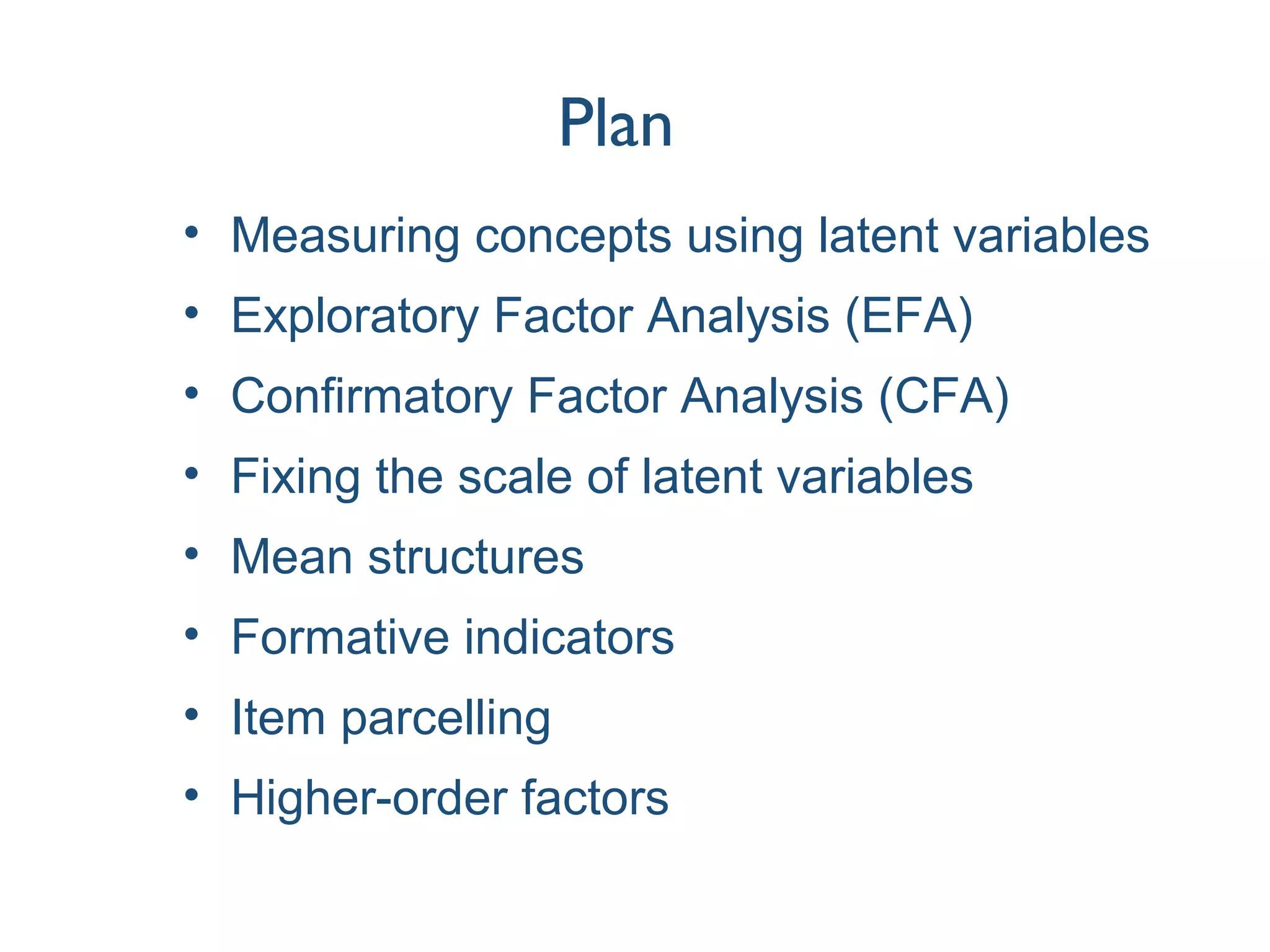
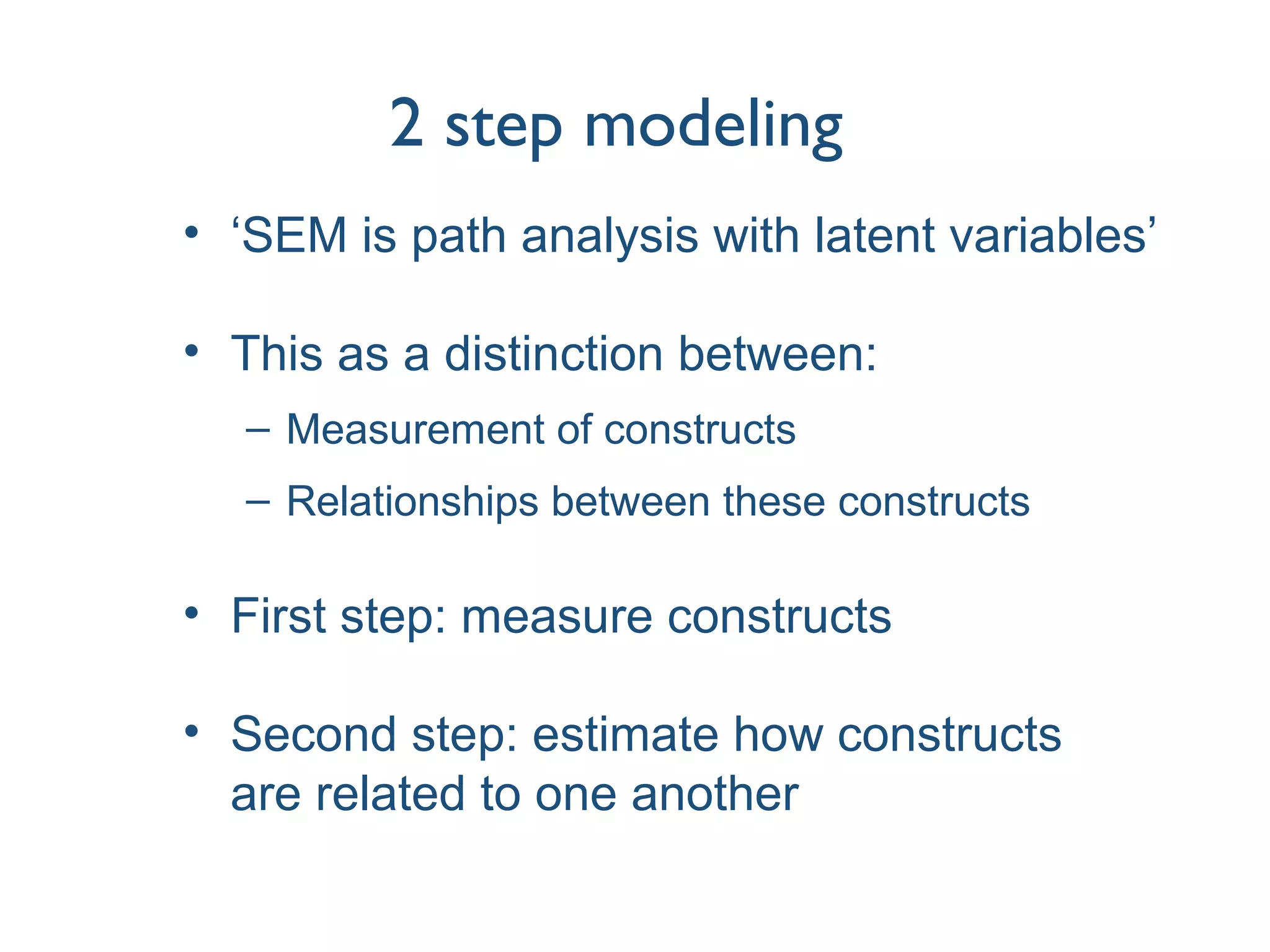
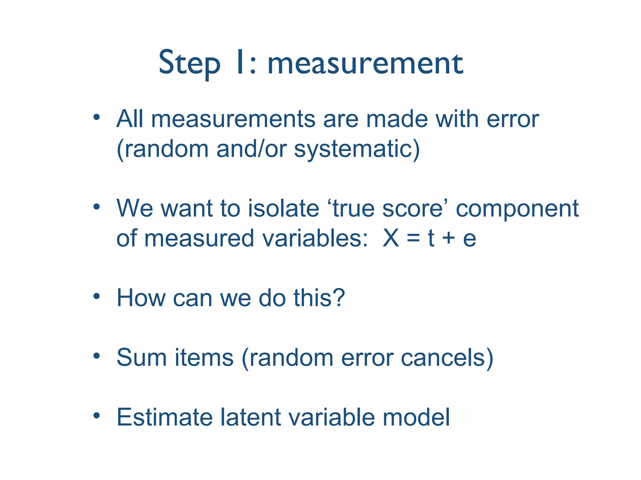
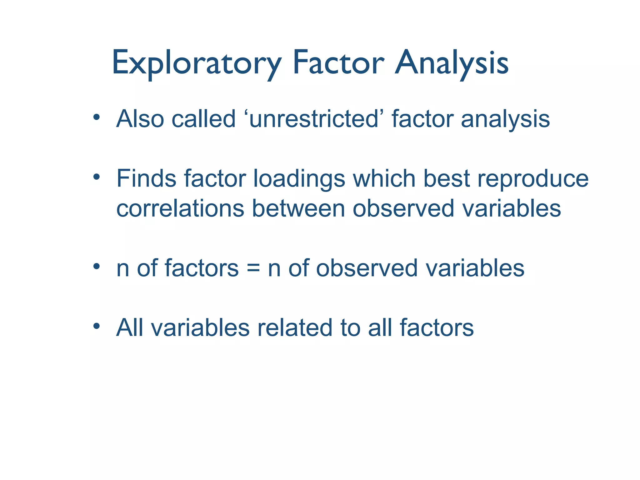
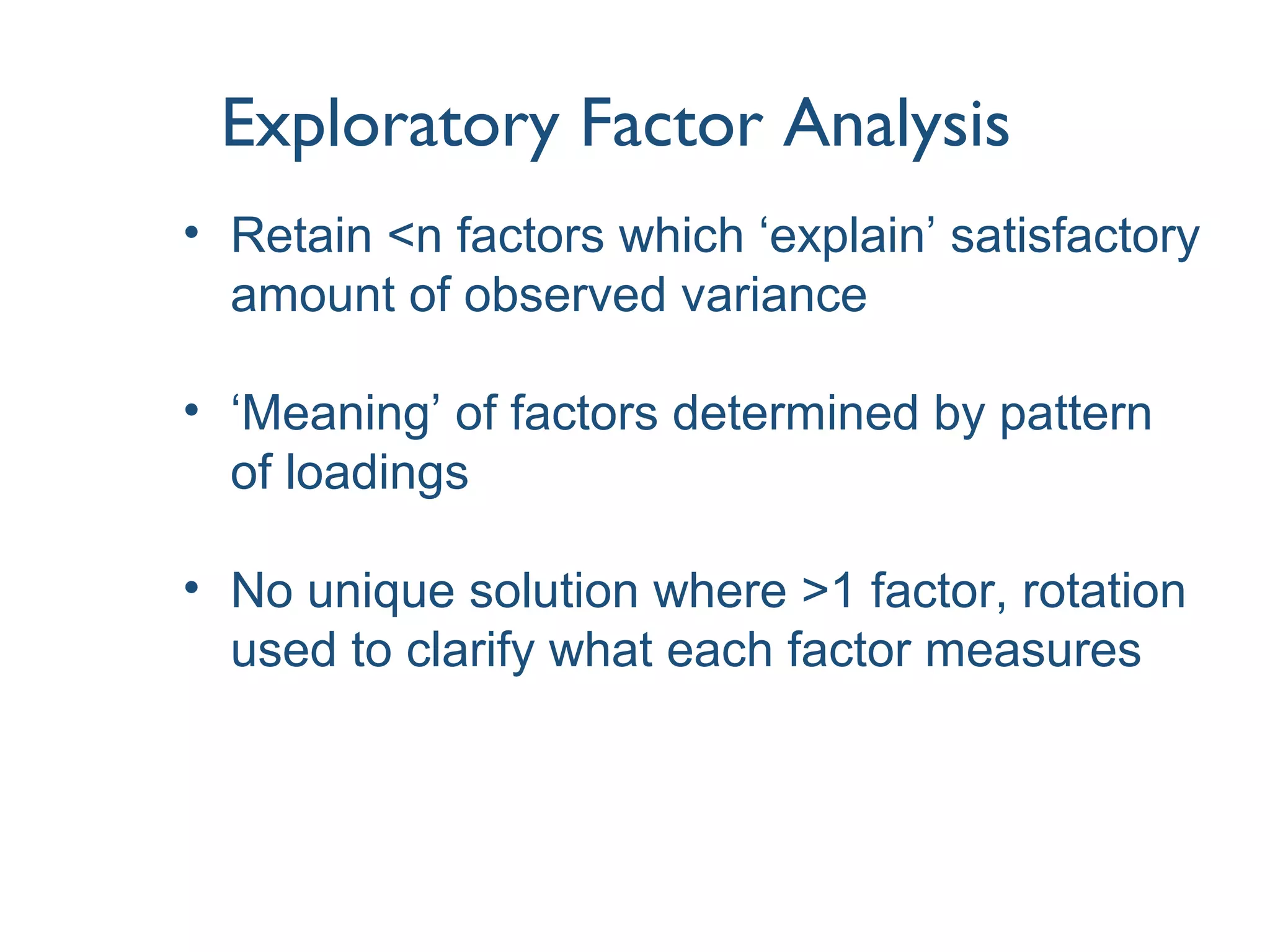
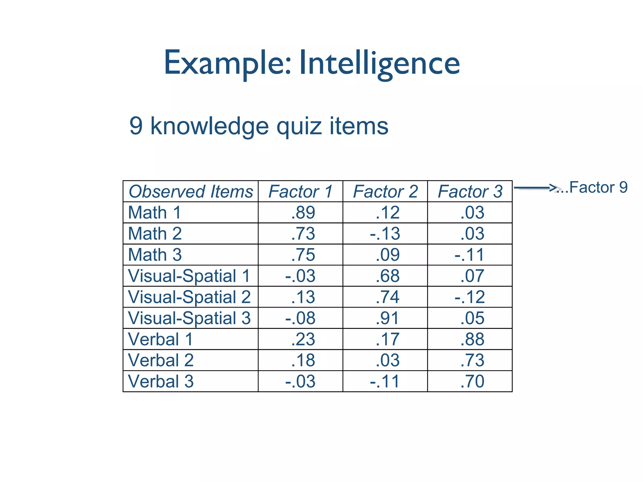
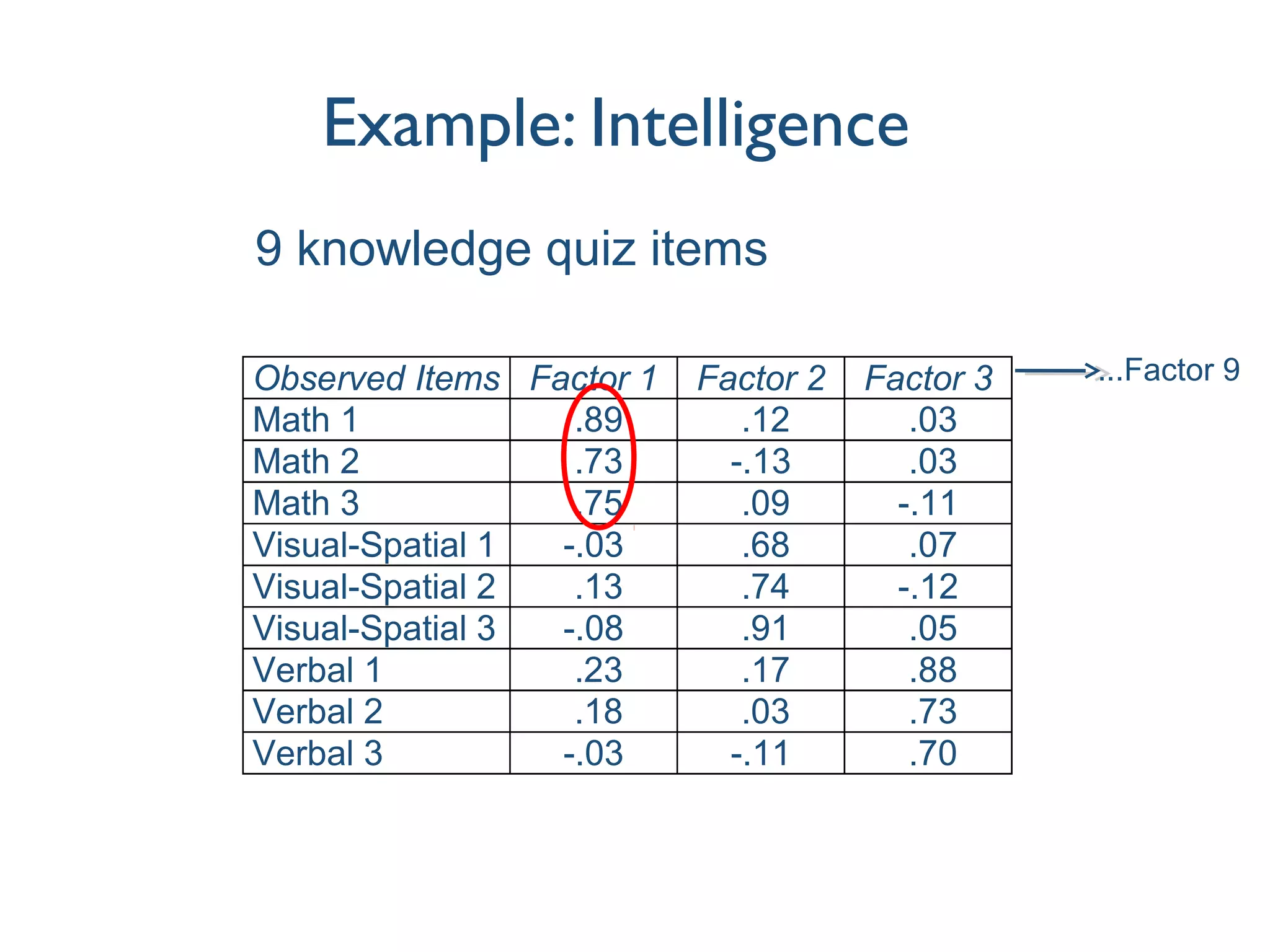
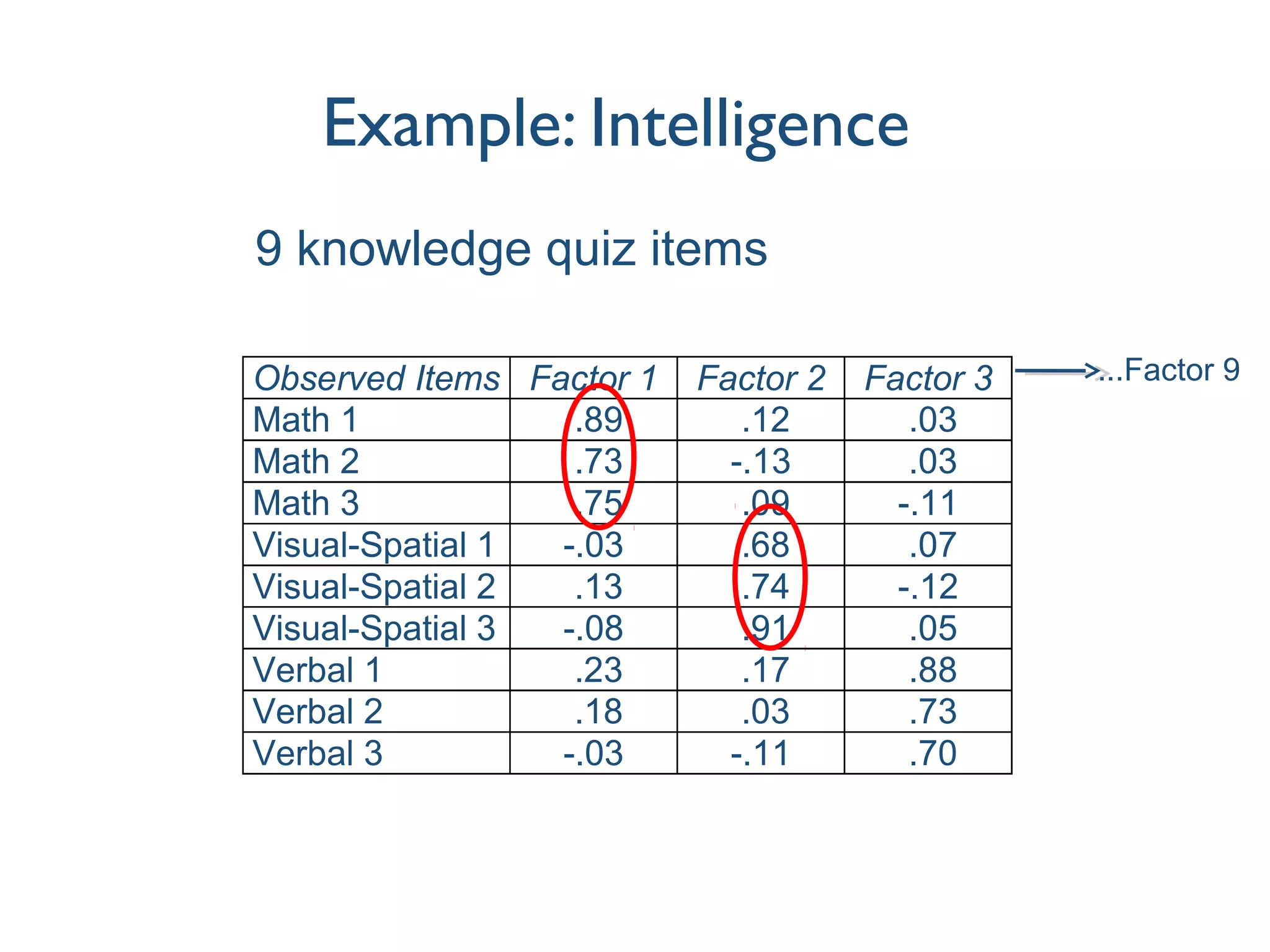
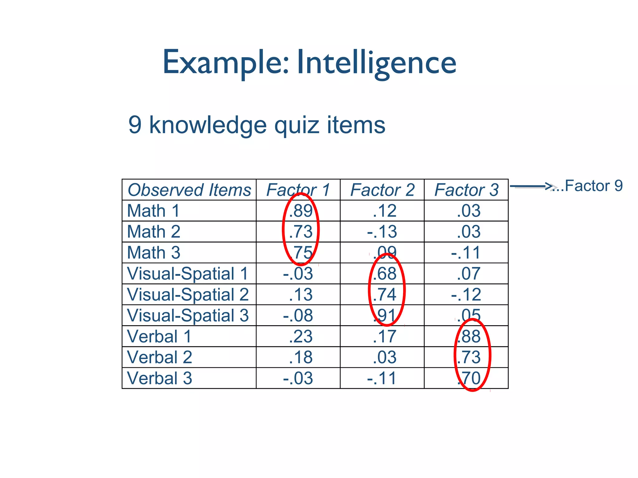
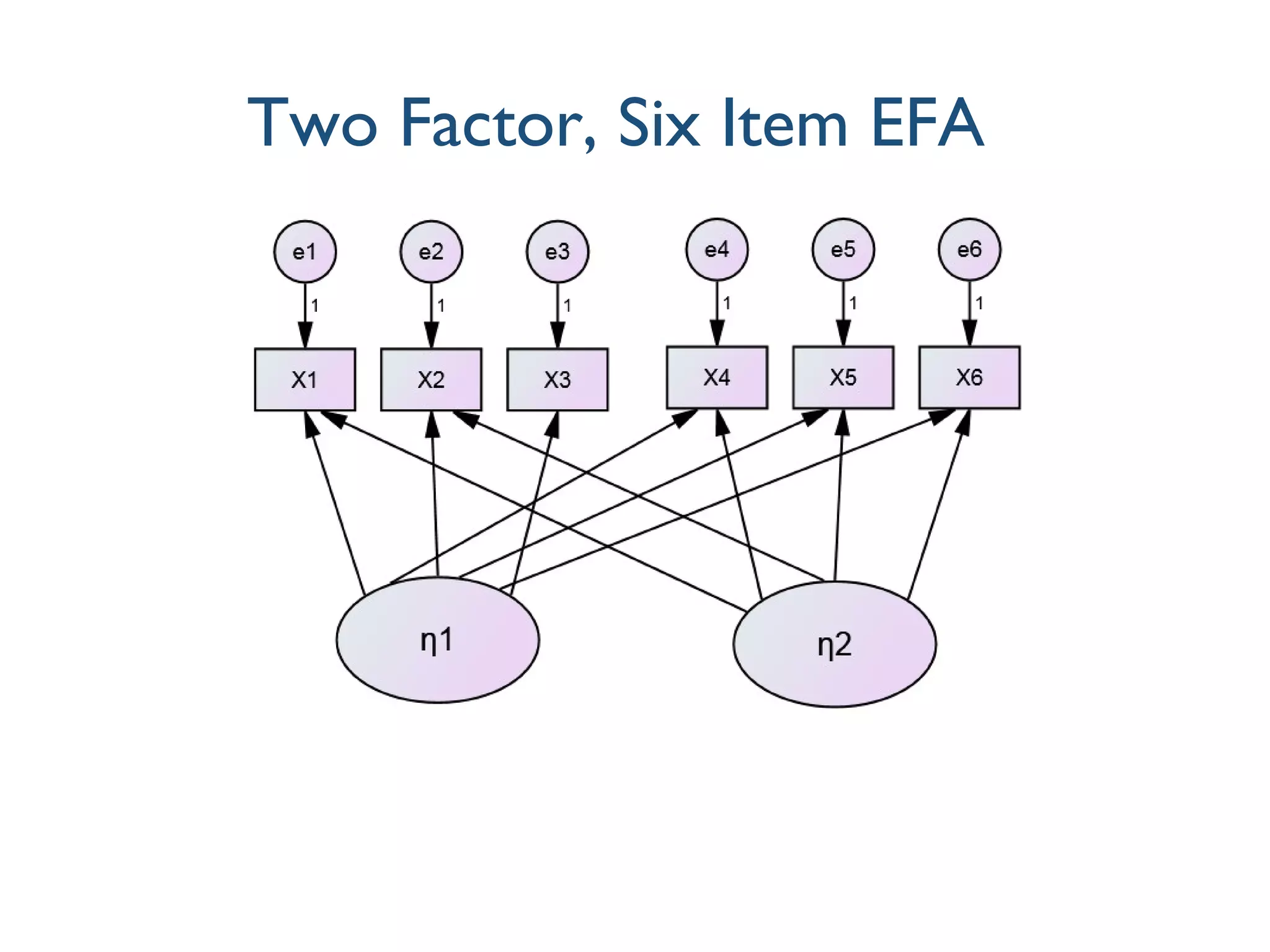
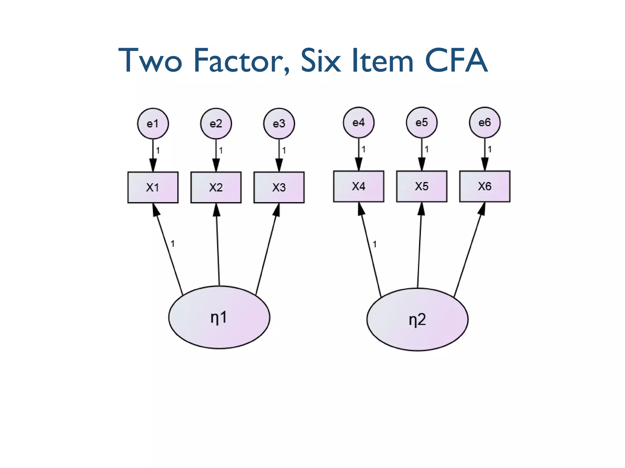
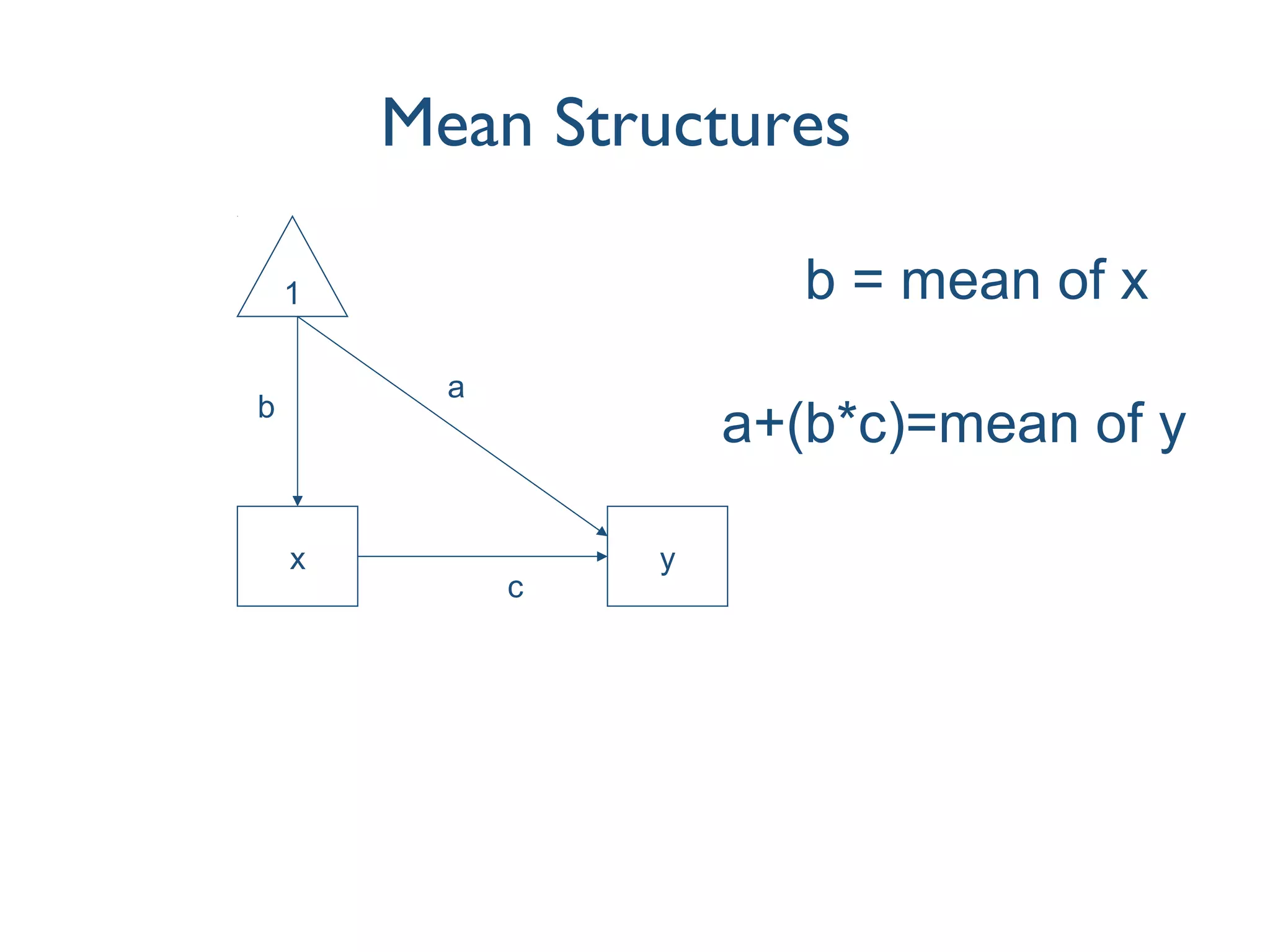
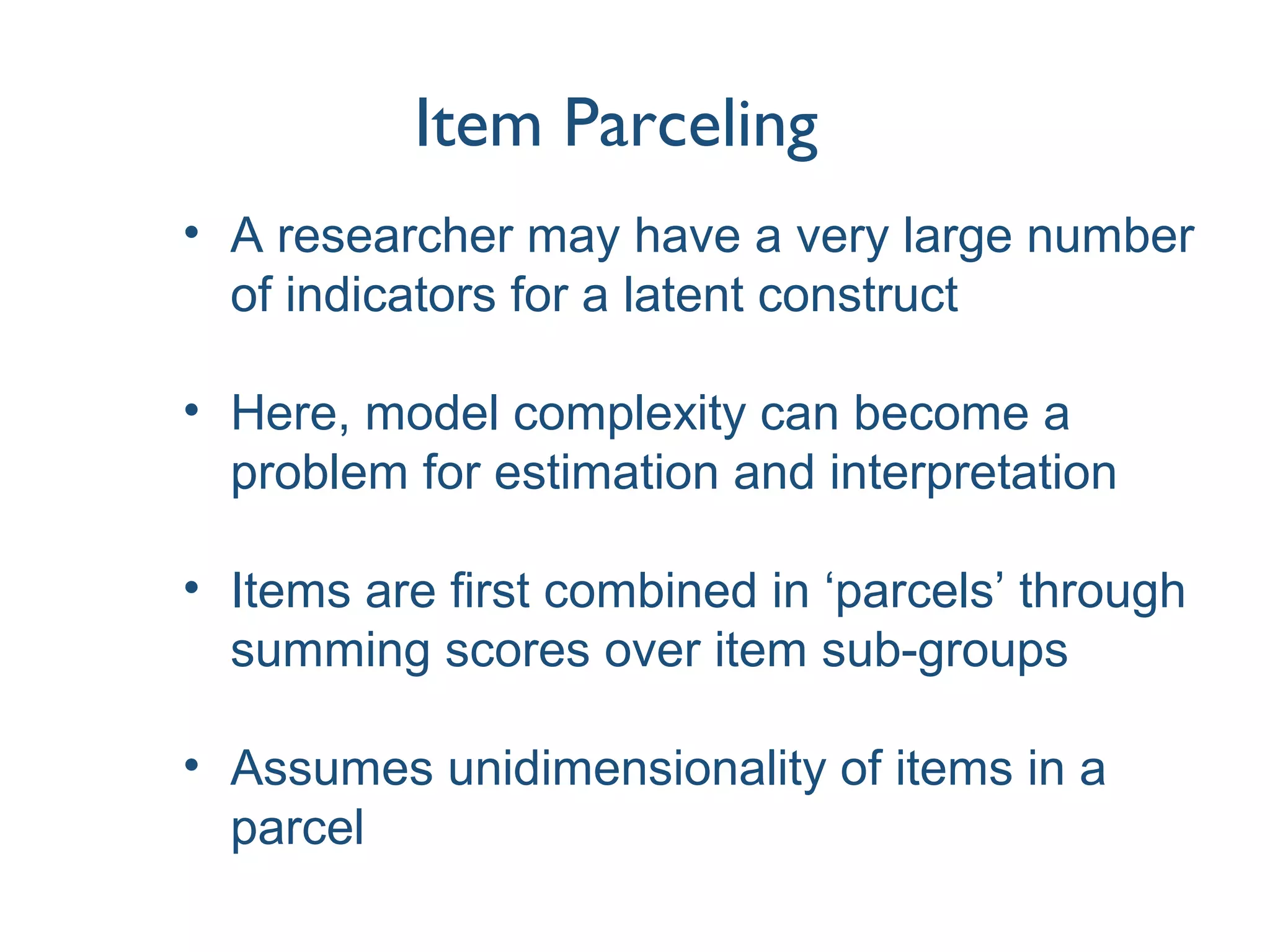
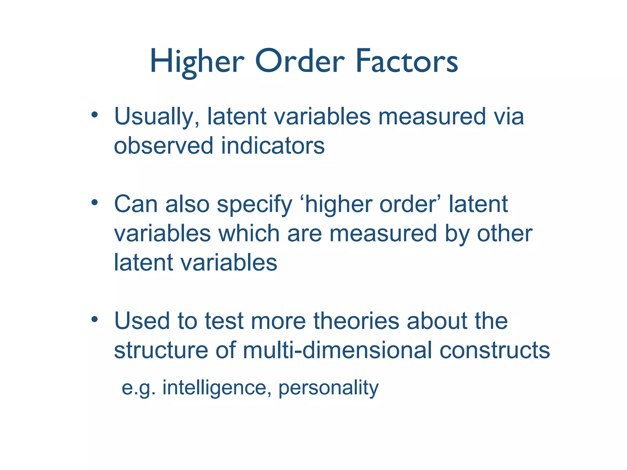
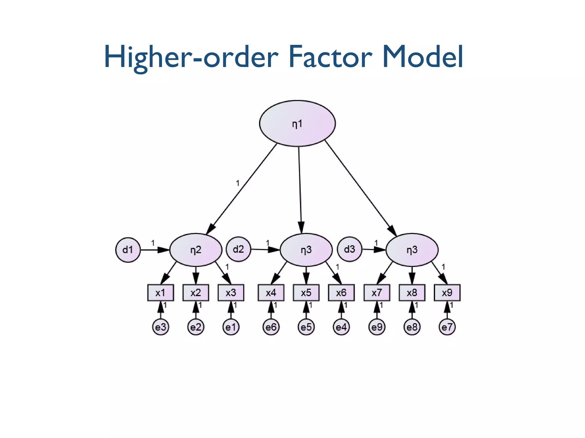
Confirmatory Factor Analysis

Confirmatory
Factor Analysis
Professor Patrick Sturgis

Plan
• Measuring concepts using latent variables
• Exploratory Factor Analysis (EFA)
• Confirmatory Factor Analysis (CFA)
• Fixing the scale of latent variables
• Mean structures
• Formative indicators
• Item parcelling
• Higher-order factors

2 step modeling
• ‘SEM is path analysis with latent variables’
• This as a distinction between:
– Measurement of constructs
– Relationships between these constructs
• First step: measure constructs
• Second step: estimate how constructs
are related to one another

Step 1: measurement
• All measurements are made with error
(random and/or systematic)
• We want to isolate ‘true score’ component
of measured variables: X = t + e
• How can we do this?
• Sum items (random error cancels)
• Estimate latent variable model

Exploratory Factor Analysis
• Also called ‘unrestricted’ factor analysis
• Finds factor loadings which best reproduce
correlations between observed variables
• n of factors = n of observed variables
• All variables related to all factors

Exploratory Factor Analysis
• Retain <n factors which ‘explain’ satisfactory
amount of observed variance
• ‘Meaning’ of factors determined by pattern
of loadings
• No unique solution where >1 factor, rotation
used to clarify what each factor measures

Example: Intelligence
Observed Items Factor 1 Factor 2 Factor 3
Math 1 .89 .12 .03
Math 2 .73 -.13 .03
Math 3 .75 .09 -.11
Visual-Spatial 1 -.03 .68 .07
Visual-Spatial 2 .13 .74 -.12
Visual-Spatial 3 -.08 .91 .05
Verbal 1 .23 .17 .88
Verbal 2 .18 .03 .73
Verbal 3 -.03 -.11 .70
9 knowledge quiz items
...Factor 9

Limitations of EFA
• Inductive, atheoretical (Data->Theory)
• Subjective judgement & heuristic rules
• We usually have a theory about how
indicators are related to particular latent
variables (Theory-> Data)
• Be explicit and test this measurement theory
against sample data

Confirmatory Factor Analysis (CFA)
• Also ‘the restricted factor model’
• Specify the measurement model before
looking at the data (the ‘no peeking’ rule!)
• Which indicators measure which factors?
• Which indicators are unrelated to which
factors?
• Are the factors correlated or uncorrelated?

Parameter Constraints
• CFA applies constraints to parameters
(hence ‘restricted’ factor model)
• Factor loadings are fixed to zero for
indicators that do not measure the factor
• Measurement theory is expressed in the
constraints that we place on the model
• Fixing parameters over-identifies the model,
can test the fit of our a priori model

Scales of latent variables
• A latent variable has no inherent metric, 2
approaches:
1. Constrain variance of latent variable to 1
2. Constrain the factor loading of one item to 1
• (2) makes item the ‘reference item’, other
loadings interpreted relative to reference
item
1. yields a standardised solution
2. generally preferred (more flexible)

Mean Structures
• In conventional SEM, we do not model
means of observed or latent variables
• Interest is in relationships between variables
(correlations, directional paths)
• Sometimes, we are interested in means of
latent variables
e.g. Differences between groups
e.g. Changes over time

Identification of latent means
• observed and latent means introduced by
adding a constant
• This is a variable set to 1 for all cases
• The regression of a variable on a predictor
and a constant, yields the intercept (mean)
of that variable in the unstandardised b
• The mean of an observed variable=total
effect of a constant on that variable

Mean Structures
x y
1
a
b
c
b = mean of x
a+(b*c)=mean of y

Means and identification
• Mean structure models require additional
identification restrictions
• We are estimating more unknown
parameters (the latent means)
• Where we have >1 group, we can fix the
latent mean of one group to zero
• Means of remaining groups are estimated
as differences from reference group

Formative and Reflective Indicators
• CFA assumes latent variable causes the
indicators, arrows point from latent to
indicator
• For some concepts this does not make
sense
e.g. using education, occupation and earnings to
measure ‘socio-economic status’
• We wouldn’t think that manipulating an
individual’s SES would change their
education

Formative Indicators
• For these latent variables, we specify the
indicators as ‘formative’
• This produces a weighted index of the
observed indicators
• Latent variable has no disturbance term
• In the path diagram, the arrows point from
indicator to latent variable

Item Parceling
• A researcher may have a very large number
of indicators for a latent construct
• Here, model complexity can become a
problem for estimation and interpretation
• Items are first combined in ‘parcels’ through
summing scores over item sub-groups
• Assumes unidimensionality of items in a
parcel

Higher Order Factors
• Usually, latent variables measured via
observed indicators
• Can also specify ‘higher order’ latent
variables which are measured by other
latent variables
• Used to test more theories about the
structure of multi-dimensional constructs
e.g. intelligence, personality

Summary
• Measuring concepts using latent variables
• Exploratory Factor Analysis (EFA)
• Confirmatory Factor Analysis (CFA)
• Fixing the scale of latent variables
• Mean structures
• Formative indicators
• Item parcelling
• Higher-order factors

for more information contact
www.ncrm.ac.uk

Confirmatory Factor Analysis

More Related Content

What's hot

Similar to Confirmatory Factor Analysis

More from University of Southampton

Recently uploaded

Confirmatory Factor Analysis

Editor's Notes