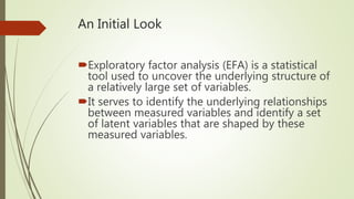
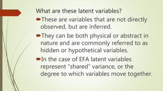
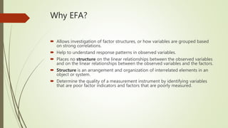
This document provides an overview of exploratory factor analysis (EFA). EFA is used to uncover the underlying structure of a set of variables and identify latent variables that are inferred rather than directly observed. It allows investigation of factor structures and helps understand response patterns. The document discusses EFA assumptions, procedures for extraction and rotation of factors, and methods for determining the appropriate number of factors.

1. An Overview:
Exploratory Factor Analysis
Daniel Briggs
North Carolina State University
January 2016

2. An Initial Look
Exploratory factor analysis (EFA) is a statistical
tool used to uncover the underlying structure of
a relatively large set of variables.
It serves to identify the underlying relationships
between measured variables and identify a set
of latent variables that are shaped by these
measured variables.

3. What are these latent variables?
These are variables that are not directly
observed, but are inferred.
They can be both physical or abstract in
nature and are commonly referred to as
hidden or hypothetical variables.
In the case of EFA latent variables
represent “shared” variance, or the
degree to which variables move together.

4. Why EFA?
 Allows investigation of factor structures, or how variables are grouped based
on strong correlations.
 Help to understand response patterns in observed variables.
 Places no structure on the linear relationships between the observed variables
and on the linear relationships between the observed variables and the factors.
 Structure is an arrangement and organization of interrelated elements in an
object or system.
 Determine the quality of a measurement instrument by identifying variables
that are poor factor indicators and factors that are poorly measured.

5. Assumptions
 Normality
 The variables have normal distributions
 In particular, we want to verify that skewness ≤ |2| and kurtosis ≤ |7|
 Linearity between variables
 Factorability
 We want to see correlation between items
 There should be some degree of collinearity among variables but not too much such that we
can still identify latent variables
 Sample size
 Sample size should be large.
 A common estimator for sufficient sample size is a large subject to variable ratio (N/k)
 The bare minimum for pilot study purposes has been reported as low as 3:1

6. Checking Factorability
Inter-item correlations (correlation matrix) - are
there at least several sizable correlations e.g., >
|.5|?
Anti-image correlation matrix diagonals - they
should be > ~.5.
Measures of sampling adequacy (MSAs):
Kaiser-Meyer-Olkin (KMO) (should be .5) and
Bartlett's test of sphericity (should be significant)

7. Fitting Procedures
Fitting procedures are used to estimate the
factor loadings and unique variances of the
model.
Factor loadings are the regression
coefficients between items and factors and
measure the influence of a common factor
on a measured variable.
All of this begins with an initial extraction.

8. Determine Number of Factors
 Issue of parsimony versus sufficiency. Overfactoring versus underfactoring.
 Researcher’s intuition
 Scree plot
 Compute the eigenvalues for the correlation matrix and plot them from smallest to largest.
 The number of eigenvalues before the last substantial drop is the number of factors.
 Eigenvalues (K1)
 Compute the eigenvalues for the correlation matrix and determine how many are greater than one.
 The number of eigenvalues greater than one corresponds to the number of factors.
 Parallel Analysis
 Create a random dataset with the same numbers of observations and variables as the original data.
 A correlation matrix is computed from the randomly generated dataset and then eigenvalues of the correlation matrix
are computed
 When the eigenvalues from the random data are larger then the eigenvalues from the initial data set then you know
that the components or factors are mostly random noise.

9. Extraction Methods
 Principal Axis Factoring (PAF)
 Considers only common variance.
 Seeks least number of factors that can account for the common variance (correlation) of a set
of variables.
 Removes the uniqueness or unexplained variability from the model.
 Principal Components Analysis (PCA)
 Considers all of the available variance.
 Seeks a linear combination of variables such that maximum variance is extracted.
 Maximum Likelihood (ML)
 Maximizes differences between factors.
 Most statistically robust

10. Rotation
 Variables load onto factors at different levels. We measure this with factor loadings.
 Factor loadings represent how much a factor affects a variable in factor analysis.
Values close to -1 and 1 indicate strong influence. Values close to 0 indicate a weak
effect.
 After factor extraction we may notice that we have difficulty interpreting and
naming the factors/components on the basis of their factor loadings.
 A solution for this difficulty is factor rotation. Factor rotation alters the pattern of
the factor loadings, and hence can improve interpretation.

11. Rotation: Types
 Orthogonal
 Orthogonal rotations constrain factors to be uncorrelated.
 An advantage of orthogonal rotation is its simplicity and conceptual clarity.
 Often there is a theoretical basis for expecting correlations amongst factors.
 Oblique
 Oblique rotations permit correlations among factors, though the factors thus identified
may not correlate.
 An advantage of oblique rotation is that it produces solutions with better simple
structure.

12. Visualizing Rotation
 Rotation can best be explained by
imagining factors as axes in a graph,
on which the original variables load.
By rotating these axes, then, it is
possible to make clusters of variables
load optimally.