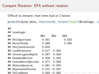
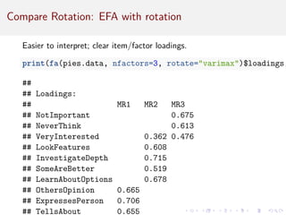
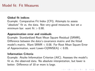
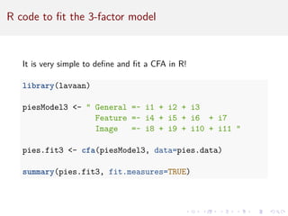
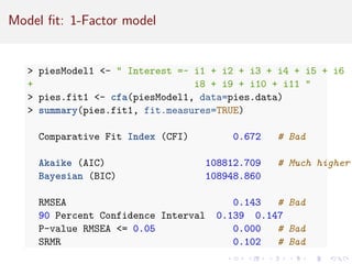
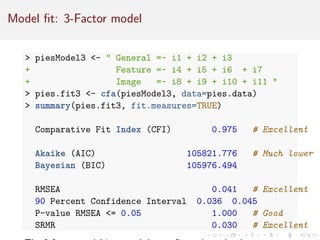
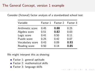
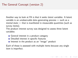
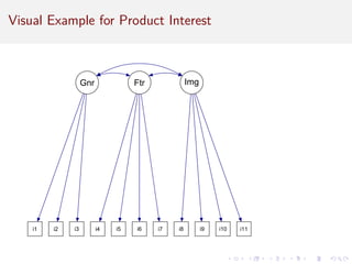
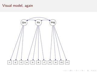
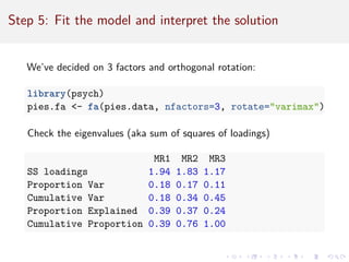
This document provides an introduction to exploratory factor analysis (EFA) and confirmatory factor analysis (CFA). It discusses the key concepts and steps in EFA, including determining the number of factors, choosing an orthogonal rotation model, interpreting the factor loadings, and using factor scores. The document provides an example EFA of 11 items from a product interest survey, finding evidence for a 3 factor solution representing image, feature, and general interest factors. Comparisons are made between EFA with rotation and principal components analysis, showing rotation improves interpretability.

1. Introduction to Factor Analysis for Marketing
SKIM/Sawtooth Software Conference 2016, Rome
Chris Chapman, Google. April 2016.
Special thanks to Josh Lewandowski at Google for helpful
feedback (errors are mine!)

2. 1 Introduction
2 Exploratory Factor Analysis
3 Does rotation work? Comparisons
4 Break!
5 Confirmatory Factor Analysis
6 Finally

3. Introduction

4. Overview
This presentation is primarily a conceptual introduction to factor
analysis. We will focus more on concepts and best practices than on
technical details.
Motivation & Basics
Exploratory Factor Analysis (EFA)
Confirmatory Factor Analysis (CFA)
Further Learning
Examples are shown in R, but the process and results are similar in
SPSS and other statistics packages.

5. Motivation: Example
Consider a standard product or satisfaction survey. These often
have multiple items for different aspects of customers’ concerns. For
example, the author’s “Product Interest and Engagement Scale” has
11 items including:
I never think about __
I am very interested in __
In choosing a __ I would look for some specific features or
options.
Some __ are clearly better than others.
When people see someone’s __ , they form an opinion of that
person.
A __ expresses a lot about the person who owns it.
It is important to choose a __ that matches one’s image.
Do these express different factors of interest?

6. Exploratory Factor Analysis

7. The General Concept (version 1)
From the original variables, factor analysis (FA) tries to find a
smaller number of derived variables (factors) that meet these
conditions:
1 Maximally capture the correlations among the original variables
(after accounting for error)
2 Each factor is associated clearly with a subset of the variables
3 Each variable is associated clearly with (ideally) only one factor
4 The factors are maximally differentiated from one another
These are rarely met perfectly in practice, but when they are
approximated, the solution is close to “simple structure” that is very
interpretable.

8. The General Concept, version 1 example
Consider (fictonal) factor analysis of a standardized school test:
Variable Factor 1 Factor 2 Factor 3
Arithmetic score 0.45 0.88 0.25
Algebra score 0.51 0.82 0.03
Logic score 0.41 0.50 0.11
Puzzle score 0.25 0.42 0.07
Vocabulary score 0.43 0.09 0.93
Reading score 0.50 0.14 0.85
We might interpret this as showing:
Factor 1: general aptitude
Factor 2: mathematical skills
Factor 3: language skills

9. The General Concept in Simplified Math
In short: the factor loading matrix, times itself (its own transpose),
closely recreates the variable-variable covariance matrix.
LL0
(+E) = C
LoadingsLoadings0
(+Error) = Covariance


F1.v1 F2.v1
F1.v2 F2.v2
F1.v3 F2.v3


F1.v1 F1.v2 F1.v3
F1.v2 F2.v2 F2.v3
=


v1.v1 v1.v2 v1.v3
v2.v1 v2.v2 v2.v3
v3.v1 v3.v2 v3.v3



10. The General Concept (version 2)
Another way to look at FA is that it seeks latent variables. A latent
variable is an unobservable data generating process — such as a
mental state — that is manifested in measurable quantities (such as
survey items).
The product interest survey was designed to assess three latent
variables:
General interest in a product category
Detailed interest in specific features
Interest in the product as an “image” product
Each of those is assessed with multiple items because any single
item is imperfect.

11. Visual Example for Product Interest
i1 i2 i3 i4 i5 i6 i7 i8 i9 i10 i11
Gnr Ftr Img

12. Very Different Modes of Factor Analysis
Exploratory Factor Analysis (EFA)
Asks what the factors are in observed data
Requires interpretation of usefulness
Before assuming it’s correct, confirm with CFA
Confirmatory Factor Analysis (CFA)
Asks how well a proposed model fits given data
Is a flavor of structural equation modeling (SEM)
Doesn’t give an absolute answer; should compare models

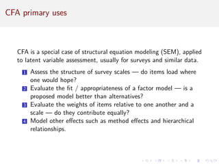
13. Key terms and symbols
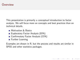
Latent variable: a presumed cognitive or data generating process
that leads to observable data. This is often a theoretical construct.
Example: Product interest. Symbol: circle/oval, such as F1 .
Manifest variable: the observed data that expresses latent
variable(s). Example: “How interested are you in this product?
[1-5]” Symbol: box, such as Item1 .
Factor: a dimensional reduction that estimates a latent variable
and its relationship to manifest variables. Example: InterestFactor.
Loading: the strength of relationship between a factor and a
variable. Example: F1 → v1 = 0.45. Ranges [-1.0 . . . 1.0], same as
Pearson’s r.

14. Visual model, again
i1 i2 i3 i4 i5 i6 i7 i8 i9 i10 i11
Gnr Ftr Img

15. EFA vs Principal Components
Factor analysis is often advantageous over PCA because:
- It’s more interpretable; FA aims for clear factor/variable
relationships
- FA does this by mathematically rotating the components to have
clearer loadings (and by omitting non-shared “error” variance)
- FA estimates latent variables in presence of error
Principal components is advantageous when:
- You want an exact reduction of the data regardless of error
- You want to maximize variance explained by the first K
components

16. General Steps for EFA
1 Load and clean the data. Put it on a common scale (e.g.,
standardize) and address extreme skew.
2 Examine correlation matrix to get a sense of possible factors
3 Determine the number of factors
4 Choose a factor rotation model (more in a moment)
5 Fit the model and interpret the resulting factors
6 Repeat 3-5 if unclear, and select the most useful
7 Use factor scores for best estimate of construct/latent variable

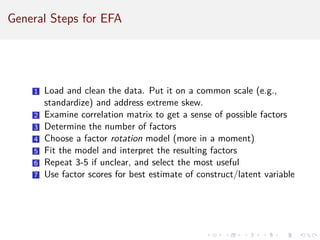
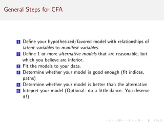
17. Now . . . data!
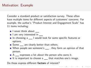
11 items for simulated product interest and engagement data
(PIES), rated on 7 point Likert type scale. We will determine the
right number of factors and their variable loadings.
Items:
Paraphrased item
not important [reversed] never think [reversed]
very interested look for specific features
investigate in depth some are clearly better
learn about options others see, form opinion
expresses person tells about person
match one’s image

18. Step 1: Load and clean data
pies.data - read.csv(http://goo.gl/yT0XwJ)
## vars n mean sd median trimmed ma
## NotImportant 1 3600 4.34 1.00 4 4.32 1.4
## NeverThink 2 3600 4.10 1.05 4 4.09 1.4
## VeryInterested 3 3600 4.11 1.02 4 4.10 1.4
## LookFeatures 4 3600 4.04 1.05 4 4.04 1.4
## InvestigateDepth 5 3600 4.00 1.08 4 4.00 1.4
## SomeAreBetter 6 3600 3.92 1.04 4 3.94 1.4
## LearnAboutOptions 7 3600 3.87 1.04 4 3.88 1.4
## OthersOpinion 8 3600 3.90 1.11 4 3.92 1.4
## ExpressesPerson 9 3600 4.02 1.01 4 4.01 1.4
## TellsAbout 10 3600 3.90 1.02 4 3.92 1.4
## MatchImage 11 3600 3.85 1.01 4 3.86 1.4
## skew kurtosis se
## NotImportant -0.07 -0.01 0.02

19. Step 2: Examine correlation matrix
Correlation plot with clustering is useful (R corrplot):
−1
−0.8
−0.6
−0.4
−0.2
0
0.2
0.4
0.6
0.8
1
NotImportant
NeverThink
VeryInterested
LookFeatures
InvestigateDepth
SomeAreBetter
LearnAboutOptions
OthersOpinion
ExpressesPerson
TellsAbout
MatchImage
NotImportant
NeverThink
VeryInterested
LookFeatures
InvestigateDepth
SomeAreBetter
LearnAboutOptions
OthersOpinion
ExpressesPerson
TellsAbout
MatchImage

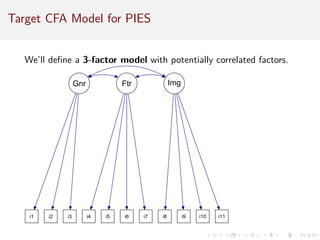
20. Step 3: Determine number of factors (1)
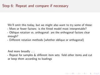
There is usually not a definitive answer. Choosing number of factors
is partially a matter of usefulness.
Generally, look for consensus among:
- Theory: how many do you expect?
- Correlation matrix: how many seem to be there?
- Eigenvalues: how many Factors have Eigenvalue 1?
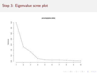
- Eigenvalue scree plot: where is the “bend” in extraction?
- Parallel analysis and acceleration [advanced; less used; not covered
today]

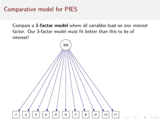
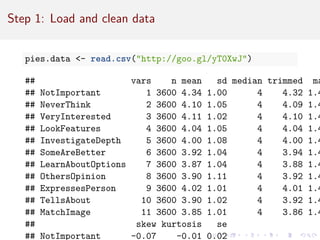
21. Step 3: Number of factors: Eigenvalues
In factor analysis, an eigenvalue is the proportion of total shared
(i.e., non-error) variance explained by each factor. You might think
of it as volume in multidimensional space, where each variable adds
1.0 to the volume (thus, sum(eigenvalues) = # of variables).
A factor is only useful if it explains more than 1 variable . . . and
thus has eigenvalue 1.0.
eigen(cor(pies.data))$values
## [1] 3.6606016 1.6422691 1.2749132 0.6880529 0.5800595 0
## [8] 0.5387749 0.5290039 0.4834441 0.4701335
This rule of thumb suggests 3 factors for the present data.

22. Step 3: Eigenvalue scree plot
prcomp(pies.data)
Variances
0.5
1.0
1.5
2.0
2.5
3.0
3.5
4.0
1 2 3 4 5 6 7 8 9 10

23. Step 4: Choose a factor rotation model
EFA can be thought of as slicing a pizza. The same material
(variance) can be carved up in ways that are mathematically
identical, but might be more or less useful for a given situation.
Key decision: do you want the extracted factors to be correlated or
not? In FA jargon, orthogonal or oblique?
By default, EFA looks for orthogonal factors that have r=0
correlation. This maximizes the interpretability, so I recommend
using an orthogonal rotation in most cases, at least to start. (As
a practical matter, it often makes little difference.)

24. Step 4: Orthogonal Rotation, Conceptually
(Figure from E. Garrett-Mayer (2006), Statistics in Psychosocial
Research. Johns Hopkins. Slides)

25. Step 4: Some rotation options
Default: varimax: orthogonal rotation that aims for clear
factor/variable structure. Generally recommended.
Oblique: oblimin: finds correlated factors while aiming for
interpretability. Recommended if you want an oblique solution.
Oblique: promax: finds correlated factors similarly, but
computationally different (good alternative). Recommended
alternative if oblimin is not available or has difficulty.
many others . . . : dozens have been developed. IMO they are
useful mostly when you’re very concerned about psychometrics
(e.g., the College Board)

26. Step 5: Fit the model and interpret the solution
We’ve decided on 3 factors and orthogonal rotation:
library(psych)
pies.fa - fa(pies.data, nfactors=3, rotate=varimax)
Check the eigenvalues (aka sum of squares of loadings)
MR1 MR2 MR3
SS loadings 1.94 1.83 1.17
Proportion Var 0.18 0.17 0.11
Cumulative Var 0.18 0.34 0.45
Proportion Explained 0.39 0.37 0.24
Cumulative Proportion 0.39 0.76 1.00

27. Step 5: Check loadings (L 0.20 shown)
A rule of thumb is to interpret loadings when |L| 0.30.
Loadings:
Factor1 Factor2 Factor3
NotImportant 0.675
NeverThink 0.614
VeryInterested 0.277 0.362 0.476
LookFeatures 0.608
InvestigateDepth 0.715
SomeAreBetter 0.519
LearnAboutOptions 0.678
OthersOpinion 0.665
ExpressesPerson 0.706
TellsAbout 0.655
MatchImage 0.632

28. Step 5: Visual representation
fa.diagram(pies.fa)
Factor Analysis
ExpressesPerson
OthersOpinion
TellsAbout
MatchImage
InvestigateDepth
LearnAboutOptions
LookFeatures
SomeAreBetter
NotImportant
NeverThink
VeryInterested
MR1
0.7
0.7
0.7
0.6
MR2
0.7
0.7
0.6
0.5
MR3
0.7
0.6
0.5

29. Step 5: Interpret
We choose names that reflect the factors:
Image Feature General
NotImportant 0.675
NeverThink 0.614
VeryInterested 0.277 0.362 0.476 # Higher order?
LookFeatures 0.608
InvestigateDepth 0.715
SomeAreBetter 0.519
LearnAboutOptions 0.678
OthersOpinion 0.665
ExpressesPerson 0.706
TellsAbout 0.655
MatchImage 0.632

30. Step 6: Repeat and compare if necessary
We’ll omit this today, but we might also want to try some of these:
- More or fewer factors: is the fitted model most interpretable?
- Oblique rotation vs. orthogonal: are the orthogonal factors clear
enough?
- Different rotation methods (whether oblique or orthogonal)
And more broadly . . .
- Repeat for samples different item sets: field other items and cut
or keep them according to loadings

31. Step 7: Use factor scores for respondents
The factor scores are the best estimate for the latent variables for
each respondent.
fa.scores - data.frame(pies.fa$scores)
names(fa.scores) - c(ImageF, FeatureF, GeneralF)
head(fa.scores)
## ImageF FeatureF GeneralF
## 1 0.5101632 -1.23897253 0.79137661
## 2 -0.0710621 0.27993881 0.66318390
## 3 -0.3044523 -0.10334393 -0.87769935
## 4 -0.8640251 -1.10904748 0.42338377
## 5 -0.6915477 -0.08739992 -0.40436752
## 6 1.5312085 -0.38443243 -0.06743736

32. Does rotation work? Comparisons

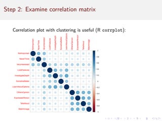
33. Compare Rotation: PCA
Difficult to interpret; item variance is spread across components.
princomp(pies.data)$loadings[ , 1:3]
## Comp.1 Comp.2 Comp.3
## NotImportant -0.2382915 0.002701817 -0.5494300
## NeverThink -0.2246788 -0.010479513 -0.6591112
## VeryInterested -0.3381471 -0.057999494 -0.2780453
## LookFeatures -0.3067349 -0.322365785 0.1806022
## InvestigateDepth -0.3345691 -0.388068434 0.1827942
## SomeAreBetter -0.2487583 -0.345378333 0.1532197
## LearnAboutOptions -0.3265734 -0.348505290 0.1168231
## OthersOpinion -0.3504562 0.395258058 0.1629491
## ExpressesPerson -0.3190419 0.340101339 0.1297465
## TellsAbout -0.3087084 0.345485125 0.1058713
## MatchImage -0.2897089 0.331665758 0.1692330

34. Compare Rotation: EFA without rotation
Difficult to interpret; most items load on 2 factors.
print(fa(pies.data, nfactors=3, rotate=none)$loadings, cu
##
## Loadings:
## MR1 MR2 MR3
## NotImportant 0.451 0.533
## NeverThink 0.386 0.495
## VeryInterested 0.609
## LookFeatures 0.517 0.334
## InvestigateDepth 0.567 0.428
## SomeAreBetter 0.406 0.324
## LearnAboutOptions 0.571 0.399
## OthersOpinion 0.581 -0.359
## ExpressesPerson 0.610 -0.387
## TellsAbout 0.569 -0.365

35. Compare Rotation: EFA with rotation
Easier to interpret; clear item/factor loadings.
print(fa(pies.data, nfactors=3, rotate=varimax)$loadings,
##
## Loadings:
## MR1 MR2 MR3
## NotImportant 0.675
## NeverThink 0.613
## VeryInterested 0.362 0.476
## LookFeatures 0.608
## InvestigateDepth 0.715
## SomeAreBetter 0.519
## LearnAboutOptions 0.678
## OthersOpinion 0.665
## ExpressesPerson 0.706
## TellsAbout 0.655

36. Break!

37. Confirmatory Factor Analysis

38. CFA primary uses
CFA is a special case of structural equation modeling (SEM), applied
to latent variable assessment, usually for surveys and similar data.
1 Assess the structure of survey scales — do items load where
one would hope?
2 Evaluate the fit / appropriateness of a factor model — is a
proposed model better than alternatives?
3 Evaluate the weights of items relative to one another and a
scale — do they contribute equally?
4 Model other effects such as method effects and hierarchical
relationships.

39. General Steps for CFA
1 Define your hypothesized/favored model with relationships of
latent variables to manifest variables.
2 Define 1 or more alternative models that are reasonable, but
which you believe are inferior.
3 Fit the models to your data.
4 Determine whether your model is good enough (fit indices,
paths)
5 Determine whether your model is better than the alternative
6 Intepret your model (Optional: do a little dance. You deserve
it!)

40. Target CFA Model for PIES
We’ll define a 3-factor model with potentially correlated factors.
i1 i2 i3 i4 i5 i6 i7 i8 i9 i10 i11
Gnr Ftr Img

41. Comparative model for PIES
Compare a 1-factor model where all variables load on one interest
factor. Our 3-factor model must fit better than this to be of
interest!
i1 i2 i3 i4 i5 i6 i7 i8 i9 i10 i11
Int

42. Model fit: Fit Measures
Global fit indices
Example: Comparative Fit Index (CFI). Attempts to assess
“absolute” fit vs. the data. Not very good measures, but set a
minimum bar: want fit 0.90.
Approximation error and residuals
Example: Standardized Root Mean Square Residual (SRMR).
Difference between the data’s covariance matrix and the fitted
model’s matrix. Want SRMR 0.08. For Root Mean Square Error
of Approximation, want Lower-CI(RMSEA) 0.05.
Information Criteria
Example: Akaike Information Criterion (AIC). Assesses the model’s
fit vs. the observed data. No absolute interpretation, but lower is
better. Difference of 10 or more is large.

43. R code to fit the 3-factor model
It is very simple to define and fit a CFA in R!
library(lavaan)
piesModel3 - General =~ i1 + i2 + i3
Feature =~ i4 + i5 + i6 + i7
Image =~ i8 + i9 + i10 + i11
pies.fit3 - cfa(piesModel3, data=pies.data)
summary(pies.fit3, fit.measures=TRUE)

44. Model fit: 1-Factor model
piesModel1 - Interest =~ i1 + i2 + i3 + i4 + i5 + i6
+ i8 + i9 + i10 + i11
pies.fit1 - cfa(piesModel1, data=pies.data)
summary(pies.fit1, fit.measures=TRUE)
Comparative Fit Index (CFI) 0.672 # Bad
Akaike (AIC) 108812.709 # Much higher
Bayesian (BIC) 108948.860
RMSEA 0.143 # Bad
90 Percent Confidence Interval 0.139 0.147
P-value RMSEA = 0.05 0.000 # Bad
SRMR 0.102 # Bad

45. Model fit: 3-Factor model
piesModel3 - General =~ i1 + i2 + i3
+ Feature =~ i4 + i5 + i6 + i7
+ Image =~ i8 + i9 + i10 + i11
pies.fit3 - cfa(piesModel3, data=pies.data)
summary(pies.fit3, fit.measures=TRUE)
Comparative Fit Index (CFI) 0.975 # Excellent
Akaike (AIC) 105821.776 # Much lower
Bayesian (BIC) 105976.494
RMSEA 0.041 # Excellent
90 Percent Confidence Interval 0.036 0.045
P-value RMSEA = 0.05 1.000 # Good
SRMR 0.030 # Excellent

46. Model Paths
Latent Variables Estimate Std.Err Z-value P(|z|)
General =~
i1 1.000
i2 0.948 0.042 22.415 0.000
i3 1.305 0.052 25.268 0.000
Feature =~
i4 1.000
i5 1.168 0.037 31.168 0.000
i6 0.822 0.033 25.211 0.000
i7 1.119 0.036 31.022 0.000
Image =~
i8 1.000
i9 0.963 0.028 34.657 0.000
i10 0.908 0.027 33.146 0.000
i11 0.850 0.027 31.786 0.000

47. Visualize it
0.20
0.22
0.23
0.82 0.85
0.91
0.95 0.96
1.00 1.00 1.00
1.12
1.17
1.31
i1 i2 i3 i4 i5 i6 i7 i8 i9 i10 i11
Gnr Ftr Img

48. A few other points on CFA
Fixing paths
To make a model identifiable, one path must be fixed between a
factor and a variable. This makes paths interpretable relative to
that variable. Standardizing predictors is important so they’re
comparable!
Modeling Factor Correlations
You might specify some factor correlations as low (e.g., 0.10) or
high (e.g., 0.50). This is easy to do in R; differs in other packages.
Hierarchical Models
You can model higher-order factors, such as overall “product
interest”. CFA allows latent variables associated with other latent
variables . . . easy, but too complex for today! (See Chapter 10 in
Chapman Feit for an example.)

49. Factor Loadings vs. Path Coefficients
By default, EFA and CFA report factor::variable coefficients on
different scales.
EFA Factor Loadings
EFA Loadings are on Pearson’s r scale, i.e., they are correlation
coefficients between the factor and the variable.
CFA Path Coefficients
CFA paths are in the variables’ own scale(s), fixed to 1.0 for one
variable per factor. If you standardize (Z-score, i.e. X−X̄
sd(X) ) variables
and fix factor variances to 1.0, they will be on the r scale. (See a
CFA reference; this is an option in many CFA packages.) Note:
Having paths on original scale is often useful in survey analysis,
because it is easy to compare to the scale itself.

50. Finally

51. The Main Points
1 If you use scales with multiple items, check them with EFA
CFA! Don’t just assume that your scales are correct, or that
items load where you expect.
2 If you have multiple item scores – such as items that add up to
a “satisfaction” score – consider using factor scores instead.
3 If you propose a complex model, prove with CFA that it’s
better than alternatives.
4 This area has a lot of jargon but is not intrinsically difficult . . .
and is much better than ignoring it and hoping for the best!
SPSS, R, SAS, and Stata all have excellent factor analysis
tools.

52. Workflow for scale development
1 Identify factors of possible interest
2 Write many items for those factors and field a survey
3 Use EFA to identify whether the factors hold up, and which
items load on them
4 Repeat 1-3 until you believe you have reliable factors and good
items
5 Use CFA to demonstrate that the factors and items hold up in
a new sample
Example: PIES scale development paper, Chapman et al, 2009

53. Learning more: Books
1 Chapman Feit (2015), R for Marketing Research and
Analytics. Chapters 8 and 10 present EFA and CFA in
marketing contexts, with detailed R code.
2 Pett, Lackey, Sullivan (2003), Making Sense of Factor
Analysis. A practical guide to EFA with emphasis on
(healthcare) survey development.
3 Brown (2015), Confirmatory Factor Analysis for Applied
Research. An excellent practical text on CFA for the social
sciences.
4 Kline (2015), Principles and Practice of Structural Equation
Modeling. The definitive guide for social science usage of CFA
and SEM.
5 DeVellis (2011), Scale Development. A very practical and
readable guide to building good survey scales.

54. Software Notes: R Packages
1 corrplot is helpful to explore correlation matrices before
attempting factor analysis.
2 psych has many options for exploratory factor analysis and
other psychometric (survey/test) applications.
3 lavaan is an easy to use SEM/CFA package. It supports
intuitive definition of models with simple equation notation.
Highly recommended.
4 semPlot makes basic SEM/CFA path diagrams as shown here.
5 DiagrammeR makes publication quality path diagrams. It
requires manual specification — tedious but not difficult — for
EFA/CFA/SEM diagrams.
6 OpenMX provides advanced options for SEM such as mixed
effects models.

55. Thank you!
Questions?
Contact: cchapman@google.com