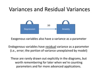
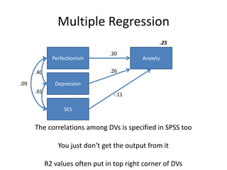
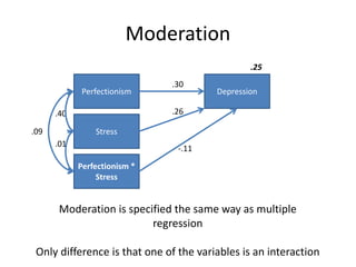
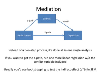
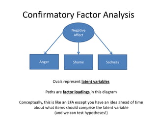
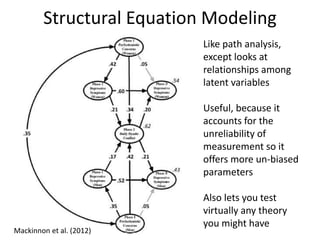
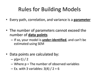
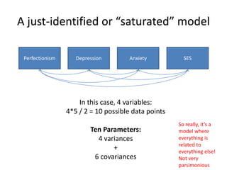
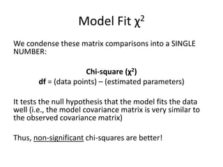
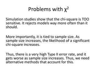
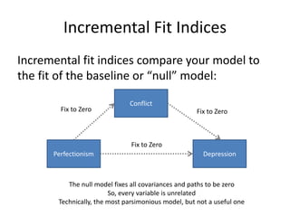
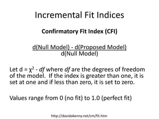
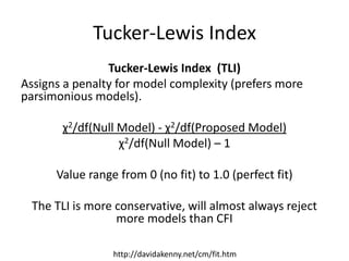
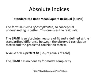
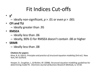
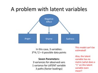
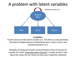
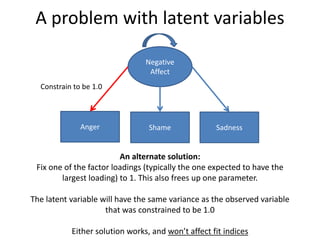
Basics of Structural Equation
Modeling
Dr. Sean P. Mackinnon
Virtually every model you’ve done already using the
Ordinary Least Squares approach (linear regression;
uses sums of squares) can also be done using SEM
The difference is primarily how the parameters and
SEs are calculated (SEM uses Maximum Likelihood
Estimation instead of Sums of Squares)
First, let’s get used to the notation of SEM diagrams
Correlation Coefficient
Depression Anxiety
.50
Rectangles indicate observed variables
Double-headed arrows indicate covariances
(so if standardized variables are used, it’s a pearson r)
Linear Regression
Depression Anxiety
.50
Single headed arrows are paths
In this example, depression is the IV and anxiety is the DV
IVs = exogenous variables (no arrows pointing to them)
DVs = endogenous variables (arrows pointing to them)
Variances and Residual Variances
Depression Anxiety
.50
Exogenous variables also have a variance as a parameter
Endogenous variables have residual variance as a parameter
(i.e., error; the portion of variance unexplained by model)
These are rarely drawn out explicitly in the diagrams, but
worth remembering for later when we’re counting
parameters and for more advanced applications.
Multiple Regression
Perfectionism Anxiety
.40
The correlations among DVs is specified in SPSS too
You just don’t get the output from it
R2 values often put in top right corner of DVs
Depression
SES
.26
-.11
.25
.09
.30
.01
Moderation
Perfectionism Depression
.40
Moderation is specified the same way as multiple
regression
Only difference is that one of the variables is an interaction
Stress
Perfectionism *
Stress
.26
-.11
.25
.09
.30
.01
Perfectionism Depression
Conflict
a-path b-path
c’-path
Instead of a two-step process, it’s done all in one single analysis
If you want to get the c-path, run one more linear regression w/o the
conflict variable included
Usually you’d use bootstrapping to test the indirect effect (a*b) in SEM
Mediation
Independent t-test
Sex Anxiety
B = 1.25
Sex is coded as 0 (women) or 1 (men)
Use unstandardized coefficents
The value for the intercept is mean for women
The value for the slope + intercept is value for men
If p-value for the slope < .05, the means are different
One-Way ANOVA (3 groups)
Treatment 1
(dummy)
Anxiety
Treatment 2
(dummy)
Original variable:
1 = Control group; 2 = Treatment 1; 3 = Treatment 2
Treatment 1 (dummy): 1 = Treatment 1, 0 = other groups
Treatment 2 (dummy): 1 = Treatment 2, 0 = other groups
Similar to the t-test, you can get means for each group
This kind of dummy coding compares treatments to the control group
SEM can also address more complicated
questions
Path Analysis
Complex relationships between variables can be used to test theory
Mackinnon et al. (2011)
Confirmatory Factor Analysis
Negative
Affect
Anger Shame Sadness
Ovals represent latent variables
Paths are factor loadings in this diagram
Conceptually, this is like an EFA except you have an idea ahead of time
about what items should comprise the latent variable
(and we can test hypotheses!)
Structural Equation Modeling
Like path analysis,
except looks at
relationships among
latent variables
Useful, because it
accounts for the
unreliability of
measurement so it
offers more un-biased
parameters
Also lets you test
virtually any theory
you might have
Mackinnon et al. (2012)
Rules for Building Models
• Every path, correlation, and variance is a parameter
• The number of parameters cannot exceed the
number of data points
– If so, your model is under-identified, and can’t be
estimated using SEM
• Data points are calculated by:
– p(p+1) / 2
– Where p = The number of observed variables
– Ex. with 3 variables: 3(4) / 2 = 6
A just-identified or “saturated” model
Perfectionism Anxiety
In this case, 4 variables:
4*5 / 2 = 10 possible data points
Ten Parameters:
4 variances
+
6 covariances
Depression SES
So really, it’s a
model where
everything is
related to
everything else!
Not very
parsimonious
Another just-identified model
Perfectionism Anxiety
In this case, 3 variables:
3*4 / 2 = 6 possible data points
Six Parameters:
3 variances
1 covariance
2 paths
Depression
Note that the
variances for
endogenous
variables will be
residual variances
(parts unexplained
by the predictors)
More Parsimonious Models
Just identified models are interesting, but often not
parsimonious (i.e., everything is related to everything)
Are there paths or covariances in your model that you
can remove, but still end up with a well-fitting model?
Path analysis and SEM can answer these questions.
When we fit models with fewer parameters than data
points, we can see if the model is still a good “fit” with
some paths omitted
An identified mediation model
Perfectionism Depression
Conflict
a-path b-path
Fix to Zero
In this case, 3 variables:
3*4 / 2 = 6 possible data points
Five Parameters:
3 variances
2 paths
(path fixed to zero has been “freed”)
Can we remove the
c’ path from this
mediation model?
This model is more
parsimonious, so it
would be preferred.
Fit indices judge the
adequacy of this
model.
Model Fit
Fit refers to the ability of a model to reproduce the data (i.e.,
usually the variance-covariance matrix).
1 2 3
1. Perfect 2.6
2. Conflict .40 5.2
3. Depression 0 .32 3.5
1 2 3
1. Perfect 2.5
2. Conflict .39 5.3
3. Depression .03 .40 3.1
Predicted by Model Actually observed in your data
So, in SEM we compare these matrices (model-created vs.
actually observed in your data), and see how discrepant they
are. If they are basically identical, the model “fits well”
Model Fit χ2
We condense these matrix comparisons into a SINGLE
NUMBER:
Chi-square (χ2)
df = (data points) – (estimated parameters)
It tests the null hypothesis that the model fits the data
well (i.e., the model covariance matrix is very similar to
the observed covariance matrix)
Thus, non-significant chi-squares are better!
Problems with χ2
Simulation studies show that the chi-square is TOO
sensitive. It rejects models way more often than it
should.
More importantly, it is tied to sample size. As
sample size increases, the likelihood of a significant
chi-square increases.
Thus, there is a very high Type II error rate, and it
gets worse as sample size increases. Thus, we need
alternative methods that account for this.
Incremental Fit Indices
Incremental fit indices compare your model to
the fit of the baseline or “null” model:
Perfectionism Depression
Conflict
Fix to Zero Fix to Zero
Fix to Zero
The null model fixes all covariances and paths to be zero
So, every variable is unrelated
Technically, the most parsimonious model, but not a useful one
Incremental Fit Indices
Confirmatory Fit Index (CFI)
d(Null Model) - d(Proposed Model)
d(Null Model)
Let d = χ2 - df where df are the degrees of freedom
of the model. If the index is greater than one, it is
set at one and if less than zero, it is set to zero.
Values range from 0 (no fit) to 1.0 (perfect fit)
http://davidakenny.net/cm/fit.htm
Tucker-Lewis Index
Tucker-Lewis Index (TLI)
Assigns a penalty for model complexity (prefers more
parsimonious models).
χ2/df(Null Model) - χ2/df(Proposed Model)
χ2/df(Null Model) – 1
Value range from 0 (no fit) to 1.0 (perfect fit)
The TLI is more conservative, will almost always reject
more models than CFI
http://davidakenny.net/cm/fit.htm
Parsimonious Indices
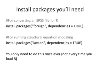
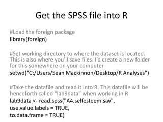
Root Mean Square Approximation of Error (RMSEA)
Similar to the others, except that it doesn’t actually
compare to the null model, and (like TLI) offers a
penalty for more complex models:
√(χ2 - df)
√[df(N - 1)]
Can also calculate a 90% CI for RMSEA
http://davidakenny.net/cm/fit.htm
Absolute Indices
Standardized Root Mean Square Residual (SRMR)
The formula is kind of complicated, so conceptual
understanding is better. This one uses the residuals.
The SRMR is an absolute measure of fit and is defined as the
standardized difference between the observed correlation
matrix and the predicted correlation matrix.
A value of 0 = perfect fit (i.e., residuals of zero)
The SRMR has no penalty for model complexity.
http://davidakenny.net/cm/fit.htm
Fit Indices Cut-offs
• χ2
– ideally non-significant, p > .01 or even p > .001
• CFI and TLI
– Ideally greater than .95
• RMSEA
– Ideally less than .06
– Ideally, 90% CI for RMSEA doesn’t contain .08 or higher
• SRMR
– Ideally less than .08
Citations for papers:
Kline, R. B. (2011). Principles and practice of structural equation modeling (3rd ed.). New
York, NY: Guilford.
Hooper, D., Coughlan, J., & Mullen, M. (2008). Structural equation modelling: guidelines for
determining model fit. Electronic Journal of Business Research Methods, 6, 53-60.
A problem with latent variables
In this case, 3 variables:
3*4 / 2 = 6 possible data points
Seven Parameters:
3 variances for observed vars
1 variance for LATENT variable
3 paths (factor loadings)
This model can’t be
estimated!
Also, the latent
variable has no
metric (what does a
“1” on this latent
variable even
mean?
Negative
Affect
Anger Shame Sadness
A problem with latent variables
A solution:
Fix the variance of the latent variable to 1. This frees up one parameter.
The latent variable becomes standardized with a mean of zero, and
standard deviation of 1.
(Actually, all along we’ve been constraining the means to be zero to
simplify the math “saturated mean structure”. Usually we don’t care
about the means for our theory so they aren’t explicitly modeled)
Constrain to be 1.0
Negative
Affect
Anger Shame Sadness
A problem with latent variables
An alternate solution:
Fix one of the factor loadings (typically the one expected to have the
largest loading) to 1. This also frees up one parameter.
The latent variable will have the same variance as the observed variable
that was constrained to be 1.0
Either solution works, and won’t affect fit indices
Constrain to be 1.0
Negative
Affect
Anger Shame Sadness
Let’s try a sample analysis in R
A confirmatory factor analysis with 10 items and
1 latent variable (general self-esteem).
Install packages you’ll need
#For converting an SPSS file for R
install.packages(“foreign", dependencies = TRUE)
#For running structural equation modeling
install.packages("lavaan", dependencies = TRUE)
You only need to do this once ever (not every time you
load R)
Get the SPSS file into R
#Load the foreign package
library(foreign)
#Set working directory to where the dataset is located.
This is also where you’ll save files. I’d create a new folder
for this somewhere on your computer
setwd("C:/Users/Sean Mackinnon/Desktop/R Analyses")
#Take the datafile and read it into R. This datafile will be
henceforth called “lab9data” when working in R
lab9data <- read.spss("A4.selfesteem.sav",
use.value.labels = TRUE,
to.data.frame = TRUE)
Specify the model
#Load the lavaan package (only need to do once per time you
open R)
library(lavaan)
#Specify the model you’re testing, call that model
“se.g.model1” (could call it anything)
#By default, will constrain the first indicator to be 1.0
se.g.model1 <-
'
se_g =~ se3 + se16r + se29 + se42r + se55 + se68 + se81r +
se94 + se107r + se120r + se131 + se135r
'
Fit the model
#Fit the data, call that fitted model “fit” (or anything you
want)
#Estimator = “MLR” is a robust estimator. I recommend
always using this instead of the default.
#missing = “ML” is to handle missing data using a full
information maximum likelihood method
#fixed.x = “TRUE” is optional. I include it because I want
results to be similar to Mplus, which is another program I
use often. See lavaan documentation for more info.
fit <- cfa(se.g.model1, data = lab9data, estimator = "MLR“,
missing = “ML”, fixed.x = “TRUE”)
Request Output
#request the summary statistics to interpret
#In this case, I request fit indices and
standardized values in addition to default output
summary(fit, fit.measures = TRUE, standardized
= TRUE)

Basics of Structural Equation Modeling

  • 1.
    Basics of StructuralEquation Modeling Dr. Sean P. Mackinnon
  • 2.
    Virtually every modelyou’ve done already using the Ordinary Least Squares approach (linear regression; uses sums of squares) can also be done using SEM The difference is primarily how the parameters and SEs are calculated (SEM uses Maximum Likelihood Estimation instead of Sums of Squares) First, let’s get used to the notation of SEM diagrams
  • 3.
    Correlation Coefficient Depression Anxiety .50 Rectanglesindicate observed variables Double-headed arrows indicate covariances (so if standardized variables are used, it’s a pearson r)
  • 4.
    Linear Regression Depression Anxiety .50 Singleheaded arrows are paths In this example, depression is the IV and anxiety is the DV IVs = exogenous variables (no arrows pointing to them) DVs = endogenous variables (arrows pointing to them)
  • 5.
    Variances and ResidualVariances Depression Anxiety .50 Exogenous variables also have a variance as a parameter Endogenous variables have residual variance as a parameter (i.e., error; the portion of variance unexplained by model) These are rarely drawn out explicitly in the diagrams, but worth remembering for later when we’re counting parameters and for more advanced applications.
  • 6.
    Multiple Regression Perfectionism Anxiety .40 Thecorrelations among DVs is specified in SPSS too You just don’t get the output from it R2 values often put in top right corner of DVs Depression SES .26 -.11 .25 .09 .30 .01
  • 7.
    Moderation Perfectionism Depression .40 Moderation isspecified the same way as multiple regression Only difference is that one of the variables is an interaction Stress Perfectionism * Stress .26 -.11 .25 .09 .30 .01
  • 8.
    Perfectionism Depression Conflict a-path b-path c’-path Insteadof a two-step process, it’s done all in one single analysis If you want to get the c-path, run one more linear regression w/o the conflict variable included Usually you’d use bootstrapping to test the indirect effect (a*b) in SEM Mediation
  • 9.
    Independent t-test Sex Anxiety B= 1.25 Sex is coded as 0 (women) or 1 (men) Use unstandardized coefficents The value for the intercept is mean for women The value for the slope + intercept is value for men If p-value for the slope < .05, the means are different
  • 10.
    One-Way ANOVA (3groups) Treatment 1 (dummy) Anxiety Treatment 2 (dummy) Original variable: 1 = Control group; 2 = Treatment 1; 3 = Treatment 2 Treatment 1 (dummy): 1 = Treatment 1, 0 = other groups Treatment 2 (dummy): 1 = Treatment 2, 0 = other groups Similar to the t-test, you can get means for each group This kind of dummy coding compares treatments to the control group
  • 11.
    SEM can alsoaddress more complicated questions
  • 12.
    Path Analysis Complex relationshipsbetween variables can be used to test theory Mackinnon et al. (2011)
  • 13.
    Confirmatory Factor Analysis Negative Affect AngerShame Sadness Ovals represent latent variables Paths are factor loadings in this diagram Conceptually, this is like an EFA except you have an idea ahead of time about what items should comprise the latent variable (and we can test hypotheses!)
  • 14.
    Structural Equation Modeling Likepath analysis, except looks at relationships among latent variables Useful, because it accounts for the unreliability of measurement so it offers more un-biased parameters Also lets you test virtually any theory you might have Mackinnon et al. (2012)
  • 15.
    Rules for BuildingModels • Every path, correlation, and variance is a parameter • The number of parameters cannot exceed the number of data points – If so, your model is under-identified, and can’t be estimated using SEM • Data points are calculated by: – p(p+1) / 2 – Where p = The number of observed variables – Ex. with 3 variables: 3(4) / 2 = 6
  • 16.
    A just-identified or“saturated” model Perfectionism Anxiety In this case, 4 variables: 4*5 / 2 = 10 possible data points Ten Parameters: 4 variances + 6 covariances Depression SES So really, it’s a model where everything is related to everything else! Not very parsimonious
  • 17.
    Another just-identified model PerfectionismAnxiety In this case, 3 variables: 3*4 / 2 = 6 possible data points Six Parameters: 3 variances 1 covariance 2 paths Depression Note that the variances for endogenous variables will be residual variances (parts unexplained by the predictors)
  • 18.
    More Parsimonious Models Justidentified models are interesting, but often not parsimonious (i.e., everything is related to everything) Are there paths or covariances in your model that you can remove, but still end up with a well-fitting model? Path analysis and SEM can answer these questions. When we fit models with fewer parameters than data points, we can see if the model is still a good “fit” with some paths omitted
  • 19.
    An identified mediationmodel Perfectionism Depression Conflict a-path b-path Fix to Zero In this case, 3 variables: 3*4 / 2 = 6 possible data points Five Parameters: 3 variances 2 paths (path fixed to zero has been “freed”) Can we remove the c’ path from this mediation model? This model is more parsimonious, so it would be preferred. Fit indices judge the adequacy of this model.
  • 20.
    Model Fit Fit refersto the ability of a model to reproduce the data (i.e., usually the variance-covariance matrix). 1 2 3 1. Perfect 2.6 2. Conflict .40 5.2 3. Depression 0 .32 3.5 1 2 3 1. Perfect 2.5 2. Conflict .39 5.3 3. Depression .03 .40 3.1 Predicted by Model Actually observed in your data So, in SEM we compare these matrices (model-created vs. actually observed in your data), and see how discrepant they are. If they are basically identical, the model “fits well”
  • 21.
    Model Fit χ2 Wecondense these matrix comparisons into a SINGLE NUMBER: Chi-square (χ2) df = (data points) – (estimated parameters) It tests the null hypothesis that the model fits the data well (i.e., the model covariance matrix is very similar to the observed covariance matrix) Thus, non-significant chi-squares are better!
  • 22.
    Problems with χ2 Simulationstudies show that the chi-square is TOO sensitive. It rejects models way more often than it should. More importantly, it is tied to sample size. As sample size increases, the likelihood of a significant chi-square increases. Thus, there is a very high Type II error rate, and it gets worse as sample size increases. Thus, we need alternative methods that account for this.
  • 23.
    Incremental Fit Indices Incrementalfit indices compare your model to the fit of the baseline or “null” model: Perfectionism Depression Conflict Fix to Zero Fix to Zero Fix to Zero The null model fixes all covariances and paths to be zero So, every variable is unrelated Technically, the most parsimonious model, but not a useful one
  • 24.
    Incremental Fit Indices ConfirmatoryFit Index (CFI) d(Null Model) - d(Proposed Model) d(Null Model) Let d = χ2 - df where df are the degrees of freedom of the model. If the index is greater than one, it is set at one and if less than zero, it is set to zero. Values range from 0 (no fit) to 1.0 (perfect fit) http://davidakenny.net/cm/fit.htm
  • 25.
    Tucker-Lewis Index Tucker-Lewis Index(TLI) Assigns a penalty for model complexity (prefers more parsimonious models). χ2/df(Null Model) - χ2/df(Proposed Model) χ2/df(Null Model) – 1 Value range from 0 (no fit) to 1.0 (perfect fit) The TLI is more conservative, will almost always reject more models than CFI http://davidakenny.net/cm/fit.htm
  • 26.
    Parsimonious Indices Root MeanSquare Approximation of Error (RMSEA) Similar to the others, except that it doesn’t actually compare to the null model, and (like TLI) offers a penalty for more complex models: √(χ2 - df) √[df(N - 1)] Can also calculate a 90% CI for RMSEA http://davidakenny.net/cm/fit.htm
  • 27.
    Absolute Indices Standardized RootMean Square Residual (SRMR) The formula is kind of complicated, so conceptual understanding is better. This one uses the residuals. The SRMR is an absolute measure of fit and is defined as the standardized difference between the observed correlation matrix and the predicted correlation matrix. A value of 0 = perfect fit (i.e., residuals of zero) The SRMR has no penalty for model complexity. http://davidakenny.net/cm/fit.htm
  • 28.
    Fit Indices Cut-offs •χ2 – ideally non-significant, p > .01 or even p > .001 • CFI and TLI – Ideally greater than .95 • RMSEA – Ideally less than .06 – Ideally, 90% CI for RMSEA doesn’t contain .08 or higher • SRMR – Ideally less than .08 Citations for papers: Kline, R. B. (2011). Principles and practice of structural equation modeling (3rd ed.). New York, NY: Guilford. Hooper, D., Coughlan, J., & Mullen, M. (2008). Structural equation modelling: guidelines for determining model fit. Electronic Journal of Business Research Methods, 6, 53-60.
  • 29.
    A problem withlatent variables In this case, 3 variables: 3*4 / 2 = 6 possible data points Seven Parameters: 3 variances for observed vars 1 variance for LATENT variable 3 paths (factor loadings) This model can’t be estimated! Also, the latent variable has no metric (what does a “1” on this latent variable even mean? Negative Affect Anger Shame Sadness
  • 30.
    A problem withlatent variables A solution: Fix the variance of the latent variable to 1. This frees up one parameter. The latent variable becomes standardized with a mean of zero, and standard deviation of 1. (Actually, all along we’ve been constraining the means to be zero to simplify the math “saturated mean structure”. Usually we don’t care about the means for our theory so they aren’t explicitly modeled) Constrain to be 1.0 Negative Affect Anger Shame Sadness
  • 31.
    A problem withlatent variables An alternate solution: Fix one of the factor loadings (typically the one expected to have the largest loading) to 1. This also frees up one parameter. The latent variable will have the same variance as the observed variable that was constrained to be 1.0 Either solution works, and won’t affect fit indices Constrain to be 1.0 Negative Affect Anger Shame Sadness
  • 32.
    Let’s try asample analysis in R A confirmatory factor analysis with 10 items and 1 latent variable (general self-esteem).
  • 33.
    Install packages you’llneed #For converting an SPSS file for R install.packages(“foreign", dependencies = TRUE) #For running structural equation modeling install.packages("lavaan", dependencies = TRUE) You only need to do this once ever (not every time you load R)
  • 34.
    Get the SPSSfile into R #Load the foreign package library(foreign) #Set working directory to where the dataset is located. This is also where you’ll save files. I’d create a new folder for this somewhere on your computer setwd("C:/Users/Sean Mackinnon/Desktop/R Analyses") #Take the datafile and read it into R. This datafile will be henceforth called “lab9data” when working in R lab9data <- read.spss("A4.selfesteem.sav", use.value.labels = TRUE, to.data.frame = TRUE)
  • 35.
    Specify the model #Loadthe lavaan package (only need to do once per time you open R) library(lavaan) #Specify the model you’re testing, call that model “se.g.model1” (could call it anything) #By default, will constrain the first indicator to be 1.0 se.g.model1 <- ' se_g =~ se3 + se16r + se29 + se42r + se55 + se68 + se81r + se94 + se107r + se120r + se131 + se135r '
  • 36.
    Fit the model #Fitthe data, call that fitted model “fit” (or anything you want) #Estimator = “MLR” is a robust estimator. I recommend always using this instead of the default. #missing = “ML” is to handle missing data using a full information maximum likelihood method #fixed.x = “TRUE” is optional. I include it because I want results to be similar to Mplus, which is another program I use often. See lavaan documentation for more info. fit <- cfa(se.g.model1, data = lab9data, estimator = "MLR“, missing = “ML”, fixed.x = “TRUE”)
  • 37.
    Request Output #request thesummary statistics to interpret #In this case, I request fit indices and standardized values in addition to default output summary(fit, fit.measures = TRUE, standardized = TRUE)