Download as PDF, PPTX

![IntroductiontoStructuralEquationModels|15May2013|KimmoVehkalahti
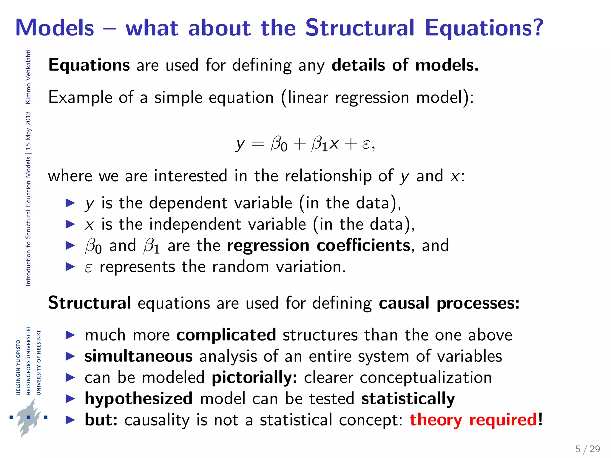
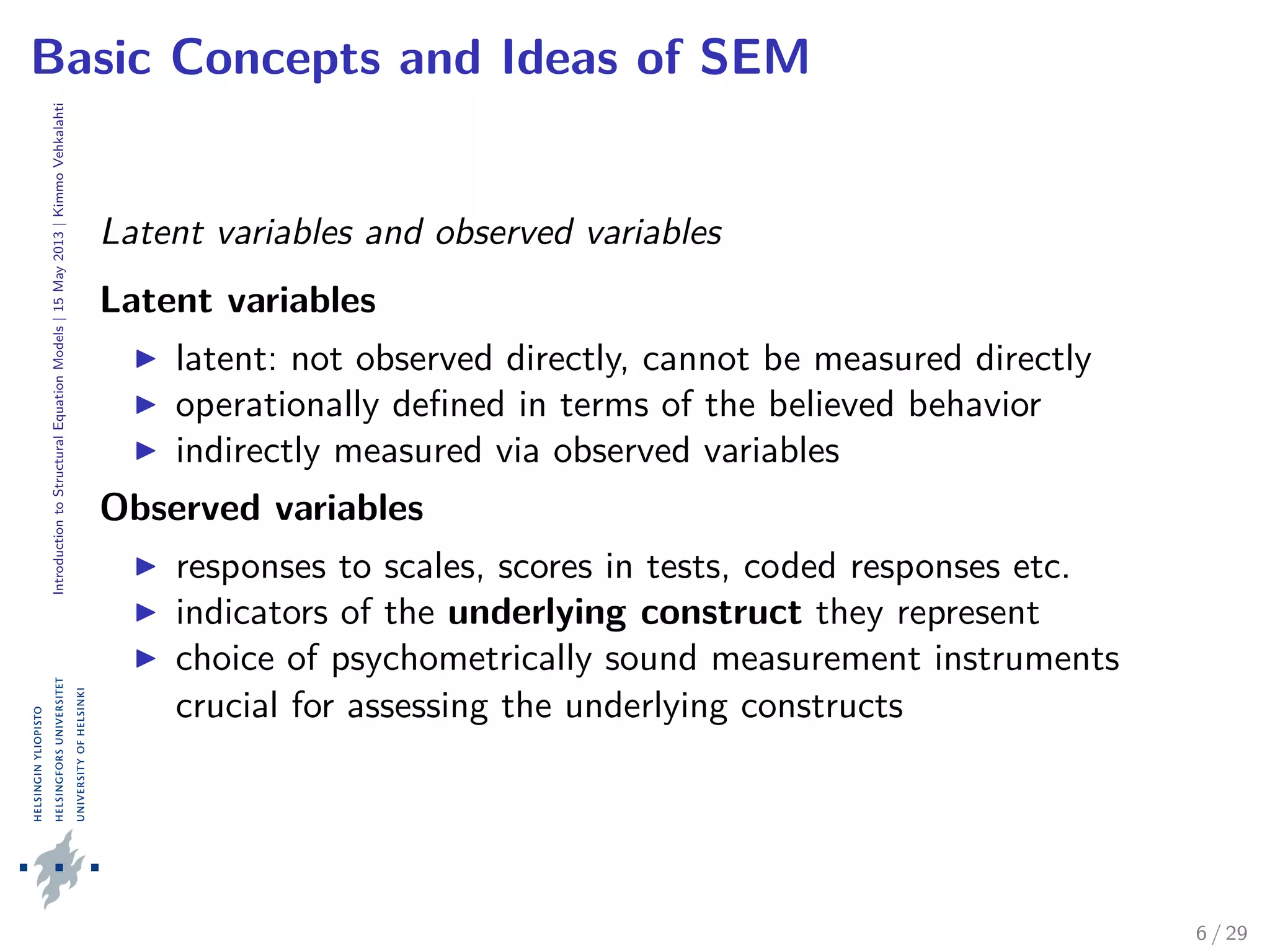
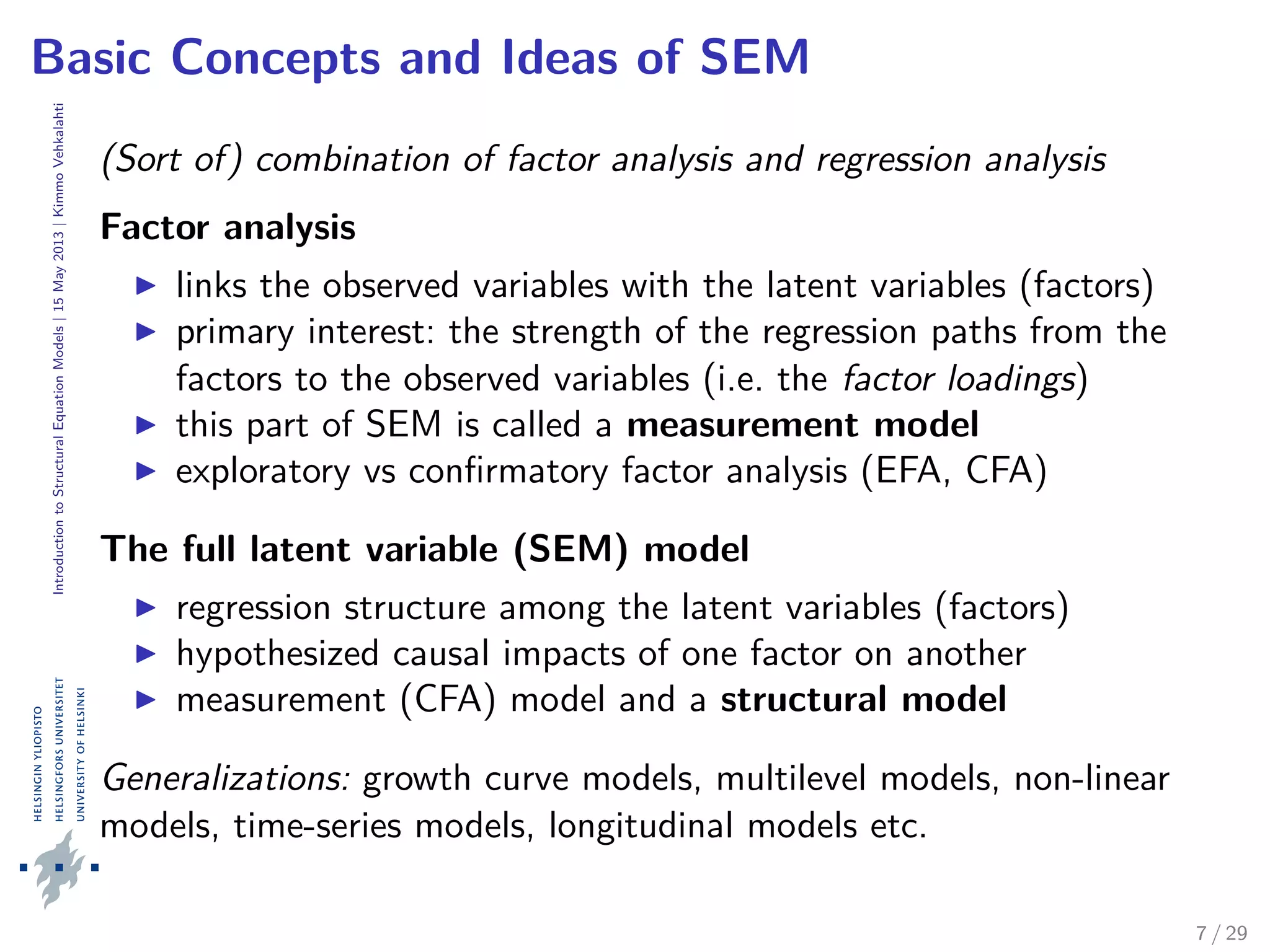
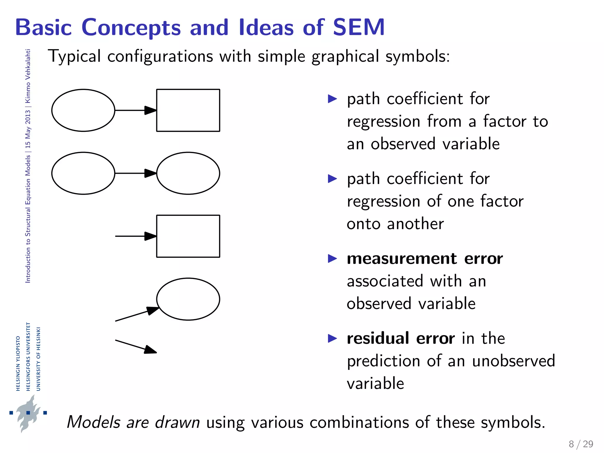
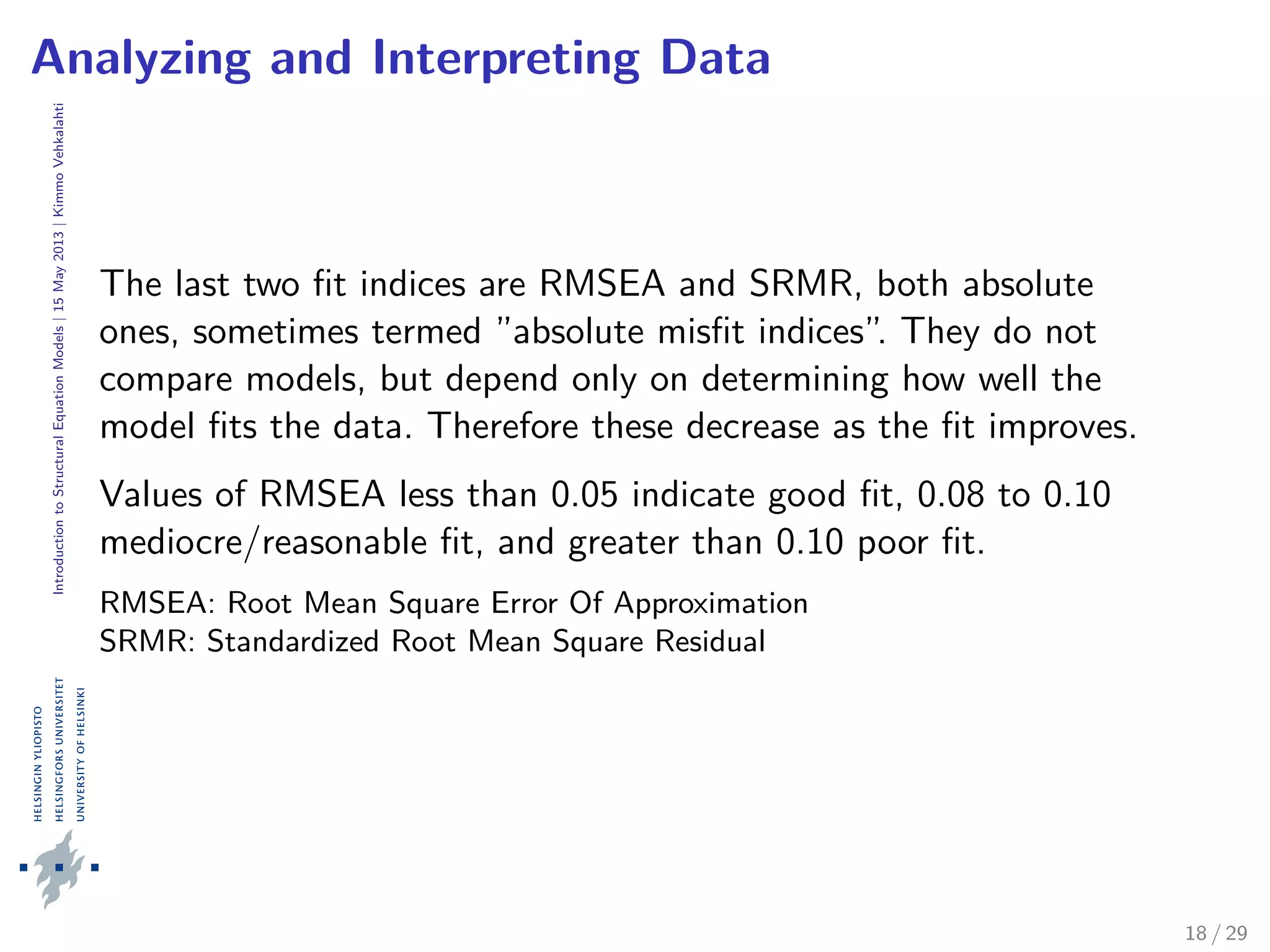
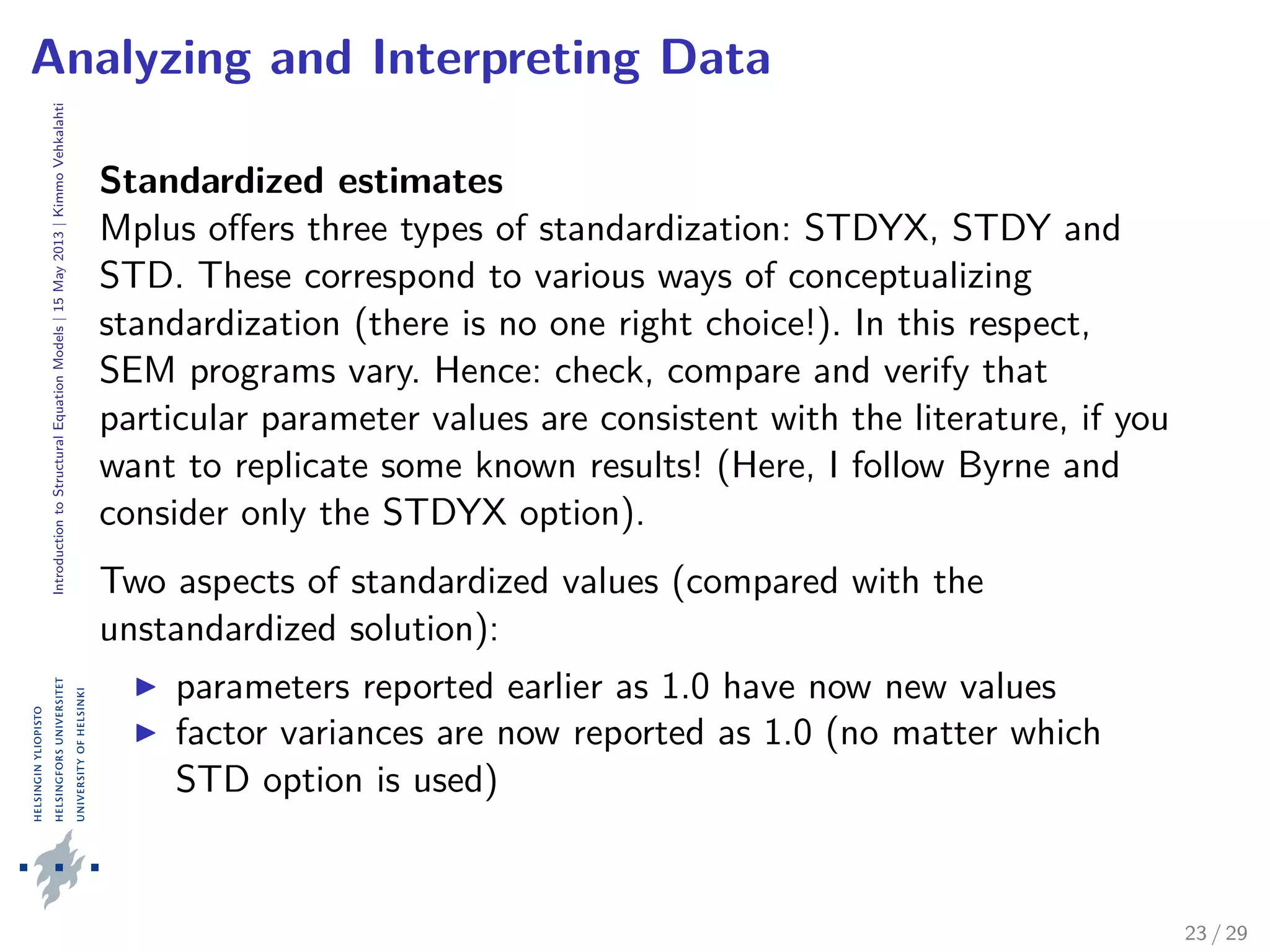
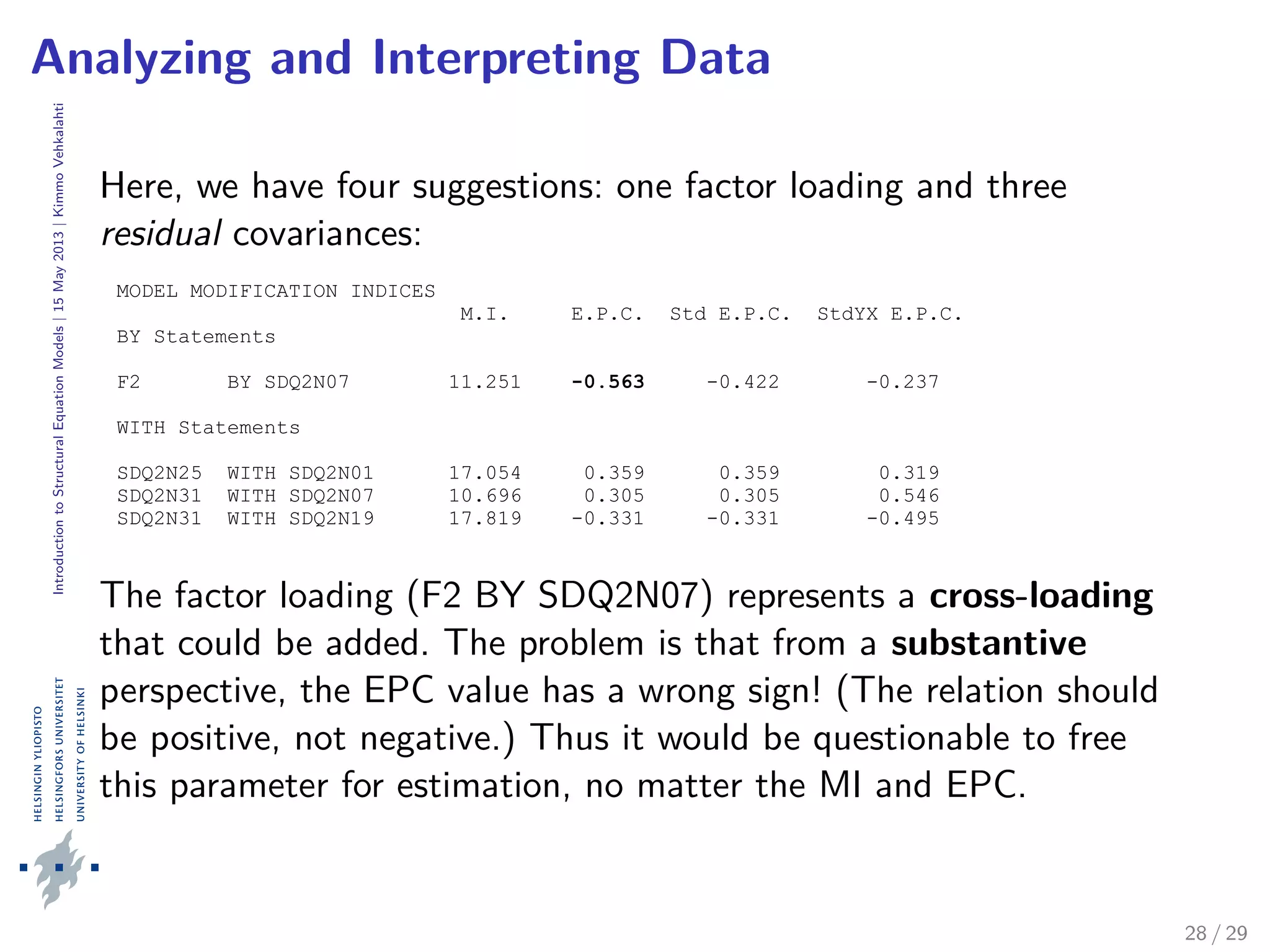
Analyzing and Interpreting Data
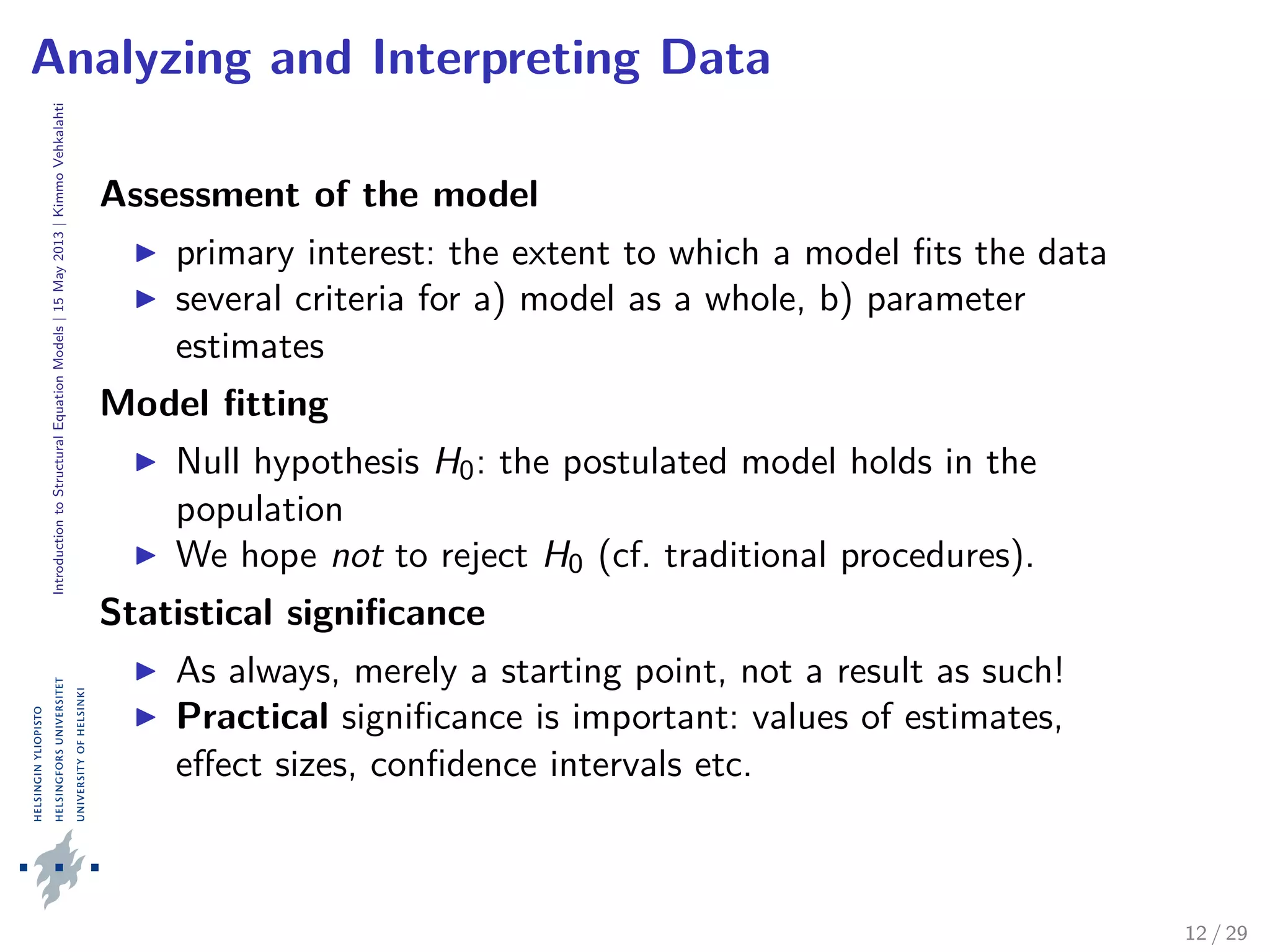
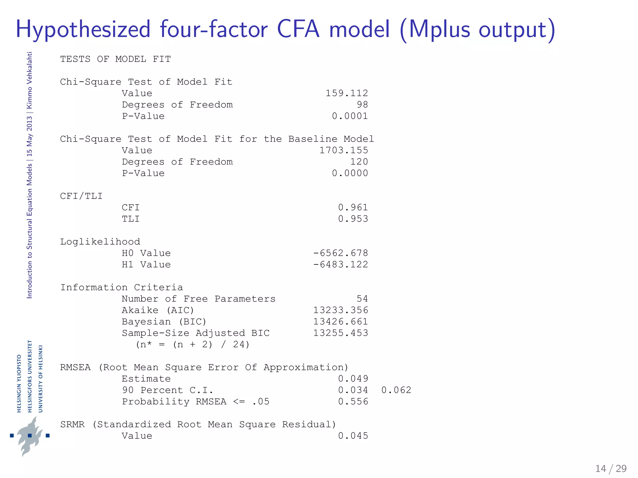
The assessment of model adequacy must be based on multiple
criteria that take into account
a) theoretical, b) statistical, and c) practical considerations.
CFI (Comparative Fit Index):
compares the hypothesized (H) and the baseline model (B)
range: [0, 1], well-fitting models have CFI > 0.95
TLI (Tucker–Lewis Fit Index):
quite similar as CFI, but nonnormed (may extend [0, 1])
includes a penalty function for overly complex models (H)
well-fitting models have TLI close to 1
17 / 29](https://image.slidesharecdn.com/structural-equation-models-introduction-kimmo-vehkalahti-2013-160504072254/75/Structural-equation-models-introduction-kimmo-vehkalahti-2013-17-2048.jpg)
![IntroductiontoStructuralEquationModels|15May2013|KimmoVehkalahti
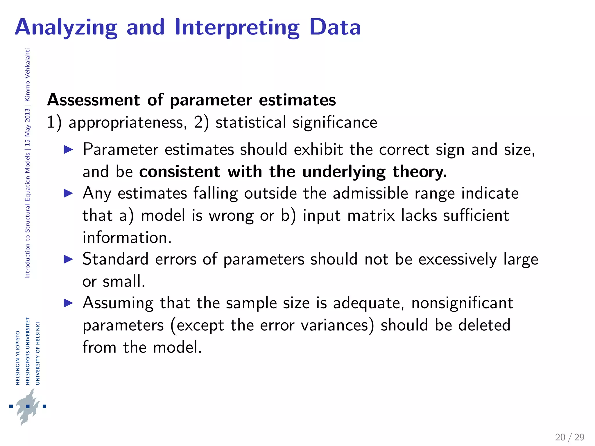
Analyzing and Interpreting Data
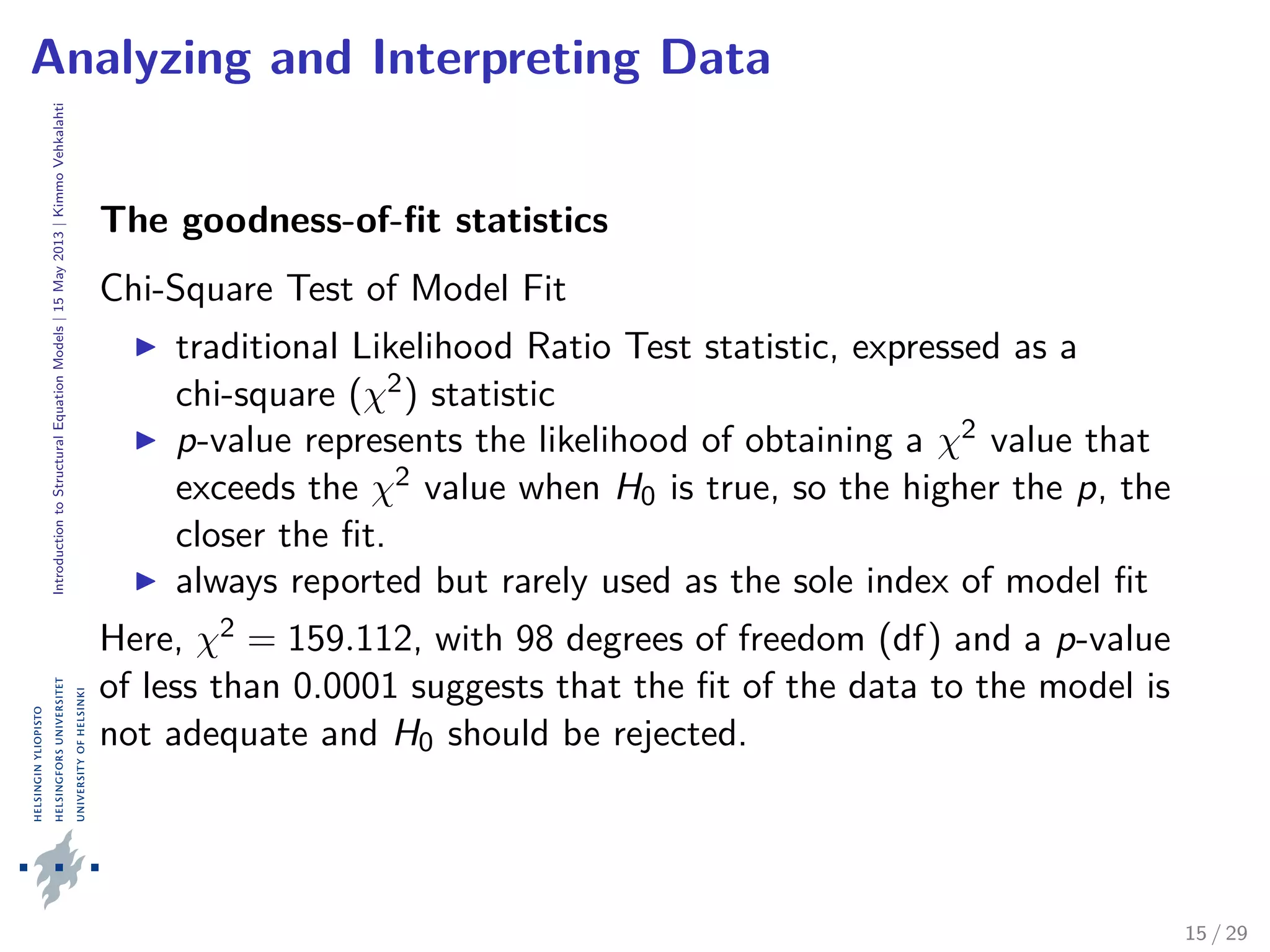
RMSEA is sensitive to the number of estimated parameters (model
complexity). Routine use of RMSEA is strongly recommended in
literature. Here: 0.049 (with a 90 % C.I. [0.034, 0.062]), indicating
a good precision.
SRMR represents the average residual value of the fit
(standardized, i.e., range [0, 1]). In well-fitting models, it will be
small, less than 0.05. Here: 0.045, that is, model explains the
correlations to within an average error of 0.045.
RMSEA: Root Mean Square Error Of Approximation
SRMR: Standardized Root Mean Square Residual
19 / 29](https://image.slidesharecdn.com/structural-equation-models-introduction-kimmo-vehkalahti-2013-160504072254/75/Structural-equation-models-introduction-kimmo-vehkalahti-2013-19-2048.jpg)
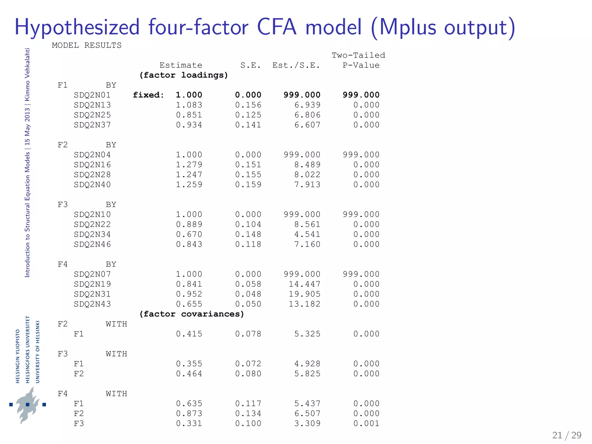
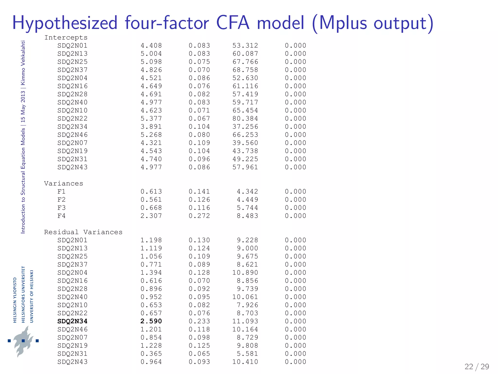

The document provides an introduction to structural equation modeling (SEM). It discusses key concepts such as latent and observed variables, and measurement models. It also presents examples of confirmatory factor analysis output to illustrate model fitting and interpretation. Specifically, it analyzes a four-factor CFA model with academic self-concept variables and reports various goodness-of-fit statistics and parameter estimates to assess how well the hypothesized model fits the sample data.