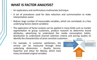
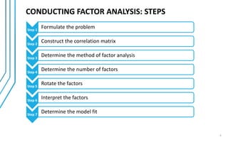
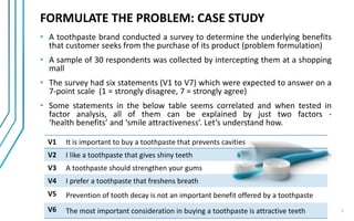
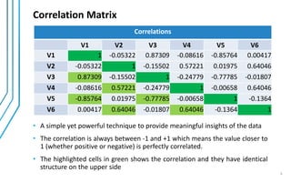
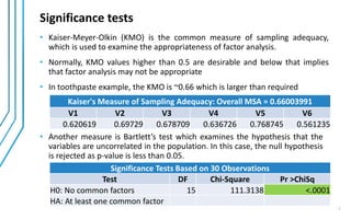
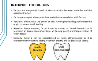
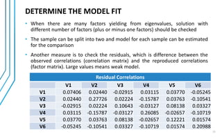
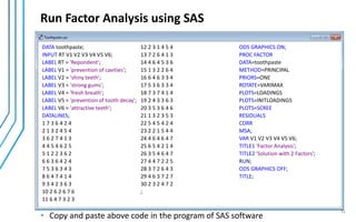
Factor analysis was conducted on survey data from 30 respondents about factors influencing toothpaste purchase. The analysis aimed to reduce the 6 survey items into underlying factors. Correlation and significance tests supported conducting factor analysis. Principal component analysis extracted 2 factors explaining over 80% of the variance: 1) "health benefits" including preventing cavities and decay and strengthening gums, and 2) "smile attractiveness" including shiny teeth and fresh breath. Varimax rotation produced a clear factor structure which was validated through model fit measures.

1. EXPLORATORY FACTOR ANALYSIS
Shailendra Tomar

2. Index
• What is Factor Analysis?
• Conducting Factor Analysis: Steps
• Formulate the problem: Case Study
• Correlation matrix
• Significance tests
• Determine the method of Factor Analysis
• Determine the number of factors
• Factor rotation methods
• Rotate the factors
• Interpret the factors
• Determine the model fit
• Run Factor Analysis using SAS 2

3. WHAT IS FACTOR ANALYSIS?
• For example, in customer satisfaction, the
service can be measured through three
underlying dimensions – Quality Service,
Expertise and Value for Money, which have
many correlated original variables
• An exploratory and confirmatory multivariate technique
• A set of procedures used for data reduction and summarization to make
interpretation easier
• Reduce large number of measurable variables, which are correlated, to a few
underlying factors (latent variables)
• The application of factor analysis can be applied in many fields such as market
segmentation to group customers, product research to determine brand
attributes, advertising to understand the media consumption habits,
distribution to understand channel selection criteria and pricing studies to
identify the characteristics of price sensitive customers.
3

4. CONDUCTING FACTOR ANALYSIS: STEPS
Step 1
Formulate the problem
Step 2
Construct the correlation matrix
Step 3
Determine the method of factor analysis
Step 4
Determine the number of factors
Step 5
Rotate the factors
Step 6
Interpret the factors
Step 7
Determine the model fit
4

5. FORMULATE THE PROBLEM: CASE STUDY
• A toothpaste brand conducted a survey to determine the underlying benefits
that customer seeks from the purchase of its product (problem formulation)
• A sample of 30 respondents was collected by intercepting them at a shopping
mall
• The survey had six statements (V1 to V7) which were expected to answer on a
7-point scale (1 = strongly disagree, 7 = strongly agree)
• Some statements in the below table seems correlated and when tested in
factor analysis, all of them can be explained by just two factors -
‘health benefits’ and ‘smile attractiveness’. Let’s understand how.
V1 It is important to buy a toothpaste that prevents cavities
V2 I like a toothpaste that gives shiny teeth
V3 A toothpaste should strengthen your gums
V4 I prefer a toothpaste that freshens breath
V5 Prevention of tooth decay is not an important benefit offered by a toothpaste
V6 The most important consideration in buying a toothpaste is attractive teeth 5

6. Correlation Matrix
Correlations
V1 V2 V3 V4 V5 V6
V1 1 -0.05322 0.87309 -0.08616 -0.85764 0.00417
V2 -0.05322 1 -0.15502 0.57221 0.01975 0.64046
V3 0.87309 -0.15502 1 -0.24779 -0.77785 -0.01807
V4 -0.08616 0.57221 -0.24779 1 -0.00658 0.64046
V5 -0.85764 0.01975 -0.77785 -0.00658 1 -0.1364
V6 0.00417 0.64046 -0.01807 0.64046 -0.1364 1
• A simple yet powerful technique to provide meaningful insights of the data
• The correlation is always between -1 and +1 which means the value closer to
1 (whether positive or negative) is perfectly correlated.
• The highlighted cells in green shows the correlation and they have identical
structure on the upper side
6

7. Significance tests
• Another measure is Bartlett’s test which examines the hypothesis that the
variables are uncorrelated in the population. In this case, the null hypothesis
is rejected as p-value is less than 0.05.
• Kaiser-Meyer-Olkin (KMO) is the common measure of sampling adequacy,
which is used to examine the appropriateness of factor analysis.
• Normally, KMO values higher than 0.5 are desirable and below that implies
that factor analysis may not be appropriate
• In toothpaste example, the KMO is ~0.66 which is larger than required
Kaiser's Measure of Sampling Adequacy: Overall MSA = 0.66003991
V1 V2 V3 V4 V5 V6
0.620619 0.69729 0.678709 0.636726 0.768745 0.561235
Significance Tests Based on 30 Observations
Test DF Chi-Square Pr >ChiSq
H0: No common factors 15 111.3138 <.0001
HA: At least one common factor
7

8. DETERMINE THE METHOD OF FACTOR ANALYSIS
• After selecting the variables for the analysis, the right method of factor
analysis should be chosen
• The most common approaches are Principal Components Analysis (PCA) and
Common & Specific Factor Analysis (CSFA)
• In PCA, the objective is to determine the minimum number of factors that will
account for maximum variance in the data. It considers the total variance
• In CSFA aka Principal Axis Factoring, the primary objective is identify the
underlying factors/dimensions and this model is based on common variance
• There are other complex methods, which requires enough statistical
experience, such as Unweighted Least Squares, Maximum Likelihood, Harris
Component Analysis, Alpha Method, and Image Factoring.
• In this example, PCA is used to define two underlying factors
8

9. DETERMINE THE NUMBER OF FACTORS
• A Priori Determination is
the first approach to
extract the factors, but in
this example, we don’t
have any prior knowledge
• Eigenvalues more than 1
will be retained as a factor
• A scree plot has plotted
eigenvalues where factors
are chosen based on steep
break on the slope
• Variance Explained plot
shows how much each
factor explain the variance
Eigenvalues of the Correlation Matrix: Total = 6 Average = 1
Eigenvalue Difference Proportion Cumulative
1 2.73118833 0.51306906 0.4552 0.4552
2 2.21811927 1.77652136 0.3697 0.8249
3 0.44159791 0.10034027 0.0736 0.8985
4 0.34125765 0.15862941 0.0569 0.9554
5 0.18262823 0.09741962 0.0304 0.9858
6 0.08520861 0.0142 1
• Referring the charts, two factors
are retained in this example,
explaining ~82% of variance
9

10. FACTOR ROTATION METHODS
• The idea behind factor rotation is have clear factor loadings, which is nothing
but the simple correlations between the variables and the factors
• The rotation also affects the proportion of variance explained by each factor,
which is also called communality
• The total communality of factors remains same, even after the rotation
• There are two types – ‘Orthogonal Rotation’ creates uncorrelated factors while
‘Oblique Rotation’ allows correlation
• Varimax rotation is the most commonly used method and minimizes the
number of variables that have high loadings on a factor.
• Other techniques are Quartimax, (Orthogonal), Equamax (Orthogonal) and
Promax (oblique)
10

11. ROTATE THE FACTORS
Factor Pattern Rotated Factor Pattern
Factor1 Factor2 Factor1* Factor2*
V1 0.92834 0.25323 V1 0.96189 -0.02663
V2 -0.30053 0.79525 V2 -0.05721 0.84821
V3 0.93618 0.13089 V3 0.93394 -0.14599
V4 -0.34158 0.78897 V4 -0.09832 0.8541
V5 -0.86876 -0.35079 V5 -0.93313 -0.08401
V6 -0.17664 0.87116 V6 0.08337 0.88497
Variance explained Variance explained
Factor1 Factor2 Factor1* Factor2*
2.731188 2.21812 2.6881106 2.261197
• In this example, Varimax is used to have clear factor loading as sometimes un-
rotated factors are not easy to interpret
• Factor 1 had higher loading on five variables and factor 2 had on four before
rotation and after rotation, loading is clearly distributed on both the factors
• Grey line is before rotation and blue line is after the rotation
11

12. INTERPRET THE FACTORS
• Factors are interpreted based on the correlation between variables and the
associated factors
• Factor pattern plot also explain how variables are correlated with factors.
• Variables, which are at the end of an axis, have higher loadings while near the
origin represent small loading
• Based on factor rotation, factor 1 can be named as ‘health benefits’ as it
represent V1 (prevention of cavities), V3 (strong gums) and V5 (prevention of
tooth decay)
• Similarly, factor 2 can be characterized as ‘smile attractiveness’ as it is
represented by V2 (shiny teeth), V4 (fresh breath) and V6 (attractive teeth).
Health
Benefits
Smile
Attractiveness
12

13. DETERMINE THE MODEL FIT
• When there are many factors yielding from eigenvalues, solution with
different number of factors (plus or minus one factors) should be checked
• The sample can be split into two and model for each sample can be estimated
for the comparison
• Another measure is to check the residuals, which is difference between the
observed correlations (correlation matrix) and the reproduced correlations
(factor matrix). Large values means weak model.
Residual Correlations
V1 V2 V3 V4 V5 V6
V1 0.07406 0.02440 -0.02915 0.03115 0.03770 -0.05245
V2 0.02440 0.27726 0.02224 -0.15787 0.03763 -0.10541
V3 -0.02915 0.02224 0.10643 -0.03127 0.08138 0.03327
V4 0.03115 -0.15787 -0.03127 0.26085 -0.02657 -0.10719
V5 0.03770 0.03763 0.08138 -0.02657 0.12221 0.01574
V6 -0.05245 -0.10541 0.03327 -0.10719 0.01574 0.20988
13

14. Run Factor Analysis using SAS
DATA toothpaste;
INPUT RT V1 V2 V3 V4 V5 V6;
LABEL RT = 'Repondent';
LABEL V1 = 'prevention of cavities';
LABEL V2 = 'shiny teeth';
LABEL V3 = 'strong gums';
LABEL V4 = 'fresh breath';
LABEL V5 = 'prevention of tooth decay';
LABEL V6 = 'attractive teeth';
DATALINES;
1 7 3 6 4 2 4
2 1 3 2 4 5 4
3 6 2 7 4 1 3
4 4 5 4 6 2 5
5 1 2 2 3 6 2
6 6 3 6 4 2 4
7 5 3 6 3 4 3
8 6 4 7 4 1 4
9 3 4 2 3 6 3
10 2 6 2 6 7 6
11 6 4 7 3 2 3
12 2 3 1 4 5 4
13 7 2 6 4 1 3
14 4 6 4 5 3 6
15 1 3 2 2 6 4
16 6 4 6 3 3 4
17 5 3 6 3 3 4
18 7 3 7 4 1 4
19 2 4 3 3 6 3
20 3 5 3 6 4 6
21 1 3 2 3 5 3
22 5 4 5 4 2 4
23 2 2 1 5 4 4
24 4 6 4 6 4 7
25 6 5 4 2 1 4
26 3 5 4 6 4 7
27 4 4 7 2 2 5
28 3 7 2 6 4 3
29 4 6 3 7 2 7
30 2 3 2 4 7 2
;
ODS GRAPHICS ON;
PROC FACTOR
DATA=toothpaste
METHOD=PRINCIPAL
PRIORS=ONE
ROTATE=VARIMAX
PLOTS=LOADINGS
PLOTS=INITLOADINGS
PLOTS=SCREE
RESIDUALS
CORR
MSA;
VAR V1 V2 V3 V4 V5 V6;
TITLE1 'Factor Analysis';
TITLE2 'Solution with 2 Factors';
RUN;
ODS GRAPHICS OFF;
TITLE;
• Copy and paste above code in the program of SAS software
14

15. Thank You