Factor Analysis

1. Factor Analysis

2.  Factor Analysis can be seen as the granddaddy
of all the multivariate techniques.
 Factor analysis is a statistical approach that
can be used to analyze interrelationships
among a large number of variables and to
explain these variables in terms of their
common underlying dimensions (factors).
 The statistical approach involves finding a way
of condensing the information contained in a
number of original variables into a smaller set
of dimensions (factors) with a minimum loss
of information.
What is factor analysis?

3.  In simple terms, FA is a method of determining
k underlying variables (factors) from n sets of
measures. k being less than n.
 It may also be called a method for extracting
common factor variance from sets of measures.
 A Factor is a construct, a hypothetical entity
underlie tests, scales & items, variate of original
variables.
 Factor Matrix can be: Factorially simple and
factorially complex (one or more than one
factor)
 Factor Matrix: aij loading a of test i on factor j
What is factor analysis?

4.  Factor analysis is used to uncover the latent
structure (dimensions) of a set of variables. It
reduces attribute space from a larger
number of variables to a smaller number of
factors and as such is a "non-dependent"
procedure (that is, it does not assume a
dependent variable is specified).
 Two Objectives:
 Data reduction and
 Data Summarization

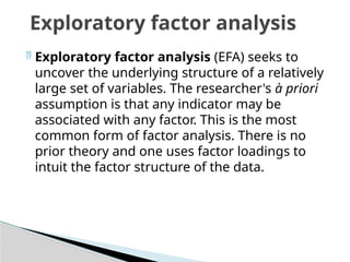
5.  Exploratory factor analysis (EFA) seeks to
uncover the underlying structure of a relatively
large set of variables. The researcher's à priori
assumption is that any indicator may be
associated with any factor. This is the most
common form of factor analysis. There is no
prior theory and one uses factor loadings to
intuit the factor structure of the data.
Exploratory factor analysis

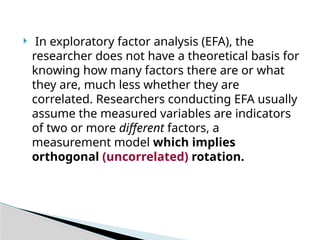
6.  In exploratory factor analysis (EFA), the
researcher does not have a theoretical basis for
knowing how many factors there are or what
they are, much less whether they are
correlated. Researchers conducting EFA usually
assume the measured variables are indicators
of two or more different factors, a
measurement model which implies
orthogonal (uncorrelated) rotation.

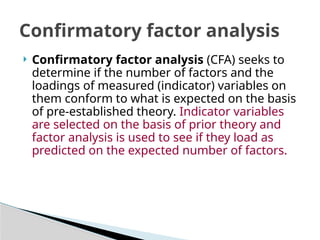
7.  Confirmatory factor analysis (CFA) seeks to
determine if the number of factors and the
loadings of measured (indicator) variables on
them conform to what is expected on the basis
of pre-established theory. Indicator variables
are selected on the basis of prior theory and
factor analysis is used to see if they load as
predicted on the expected number of factors.
Confirmatory factor analysis

8.  Factor analysis could be used to verify your
conceptualization of a construct of interest. For
example, in many studies, the construct of
“leadership" has been observed to be composed
of "task skills" and "people skills." Let's say that,
for some reason, you are developing a new
questionnaire about leadership and you create 20
items. You think 10 will reflect "task" elements
and 10 "people" elements, but since your items
are new, you want to test your conceptualization
(this is called confirmatory factor analysis).

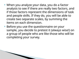
9.  When you analyze your data, you do a factor
analysis to see if there are really two factors, and
if those factors represent the dimensions of task
and people skills. If they do, you will be able to
create two separate scales, by summing the
items on each dimension.
 Before you use the questionnaire on your
sample, you decide to pretest it (always wise!) on
a group of people who are like those who will be
completing your survey.

10.  This family of techniques uses an estimate
of common variance among the original
variables to generate the factor solution.
Because of this, the number of factors will
always be less than the number of original
variables.
 Mostly used for questionnaires that are
Likert-based.

11. There are four basic factor analysis steps:
 Data collection and generation of the
correlation matrix
 Extraction of initial factor solution
 Rotation and interpretation
 Construction of scales or factor scores to use
in further analyses
 The output of a factor analysis will give you
several things. The following table shows how
output helps to determine the number of
components/factors to be retained for further
analysis.

12.  One good rule of thumb for determining the
number of factors, is the "eigenvalue greater
than 1" criteria. For the moment, let's not
worry about the meaning of eigenvalues,
however this criteria allows us to be fairly sure
that any factors we keep will account for at
least the variance of one of the variables used
in the analysis.
 There are other criteria for selecting the
number of factors to keep, but this is the
easiest to apply, since it is the default of most
statistical computer programs.
 Note that the factors will all be orthogonal to
one another, meaning that they will be

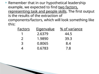
13.  Remember that in our hypothetical leadership
example, we expected to find two factors,
representing task and people skills. The first output
is the results of the extraction of
components/factors, which will look something like
this:
Factors Eigenvalue % of variance
1 2.6379 44.5
2 1.9890 39.3
3 0.8065 8.4
4 0.6783 7.8

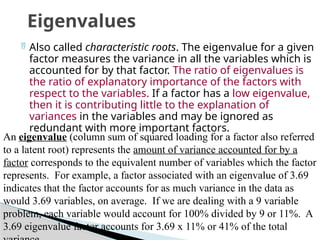
14.  Also called characteristic roots. The eigenvalue for a given
factor measures the variance in all the variables which is
accounted for by that factor. The ratio of eigenvalues is
the ratio of explanatory importance of the factors with
respect to the variables. If a factor has a low eigenvalue,
then it is contributing little to the explanation of
variances in the variables and may be ignored as
redundant with more important factors.
Eigenvalues
An eigenvalue (column sum of squared loading for a factor also referred
to a latent root) represents the amount of variance accounted for by a
factor corresponds to the equivalent number of variables which the factor
represents. For example, a factor associated with an eigenvalue of 3.69
indicates that the factor accounts for as much variance in the data as
would 3.69 variables, on average. If we are dealing with a 9 variable
problem, each variable would account for 100% divided by 9 or 11%. A
3.69 eigenvalue factor accounts for 3.69 x 11% or 41% of the total

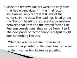
15.  Since the first two factors were the only ones
that had eigenvalues > 1, the final factor
solution will only represent 83.8% of the
variance in the data. The loadings listed under
the "Factor" headings represent a correlation
between that item and the overall factor. Like
Pearson correlations, they range from -1 to 1.
The next panel of factor analysis output might
look something like this:
While we want to account for as much
variance as possible, at the same time we want
to do it with as few factors as possible.

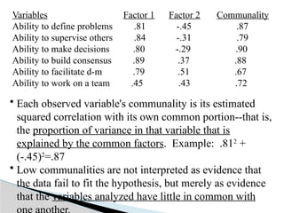
16. Variables Factor 1 Factor 2 Communality
Ability to define problems .81 -.45 .87
Ability to supervise others .84 -.31 .79
Ability to make decisions .80 -.29 .90
Ability to build consensus .89 .37 .88
Ability to facilitate d-m .79 .51 .67
Ability to work on a team .45 .43 .72
• Each observed variable's communality is its estimated
squared correlation with its own common portion--that is,
the proportion of variance in that variable that is
explained by the common factors. Example: .812
+
(-.45)2
=.87
• Low communalities are not interpreted as evidence that
the data fail to fit the hypothesis, but merely as evidence
that the variables analyzed have little in common with

17.  The sum of the squared factor loadings for all
factors for a given variable (row) is the
variance in that variable accounted for by all
the factors, and this is called the communality.
 Communality, h2, is the squared multiple
correlation for the variable using the factors
as predictors. The communality measures the
percent of variance in a given variable
explained by all the factors jointly and may be
interpreted as the reliability of the indicator.
 . Factor loadings are the basis for imputing a
label to the different factors.

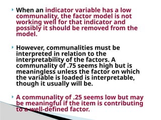
18.  When an indicator variable has a low
communality, the factor model is not
working well for that indicator and
possibly it should be removed from the
model.
 However, communalities must be
interpreted in relation to the
interpretability of the factors. A
communality of .75 seems high but is
meaningless unless the factor on which
the variable is loaded is interpretable,
though it usually will be.
 A communality of .25 seems low but may
be meaningful if the item is contributing
to a well-defined factor.

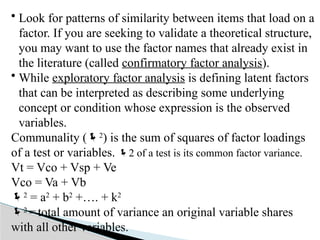
19. • Look for patterns of similarity between items that load on a
factor. If you are seeking to validate a theoretical structure,
you may want to use the factor names that already exist in
the literature (called confirmatory factor analysis).
• While exploratory factor analysis is defining latent factors
that can be interpreted as describing some underlying
concept or condition whose expression is the observed
variables.
Communality (2
) is the sum of squares of factor loadings
of a test or variables. 2 of a test is its common factor variance.
Vt = Vco + Vsp + Ve
Vco = Va + Vb
2
= a2
+ b2
+…. + k2
2
=total amount of variance an original variable shares
with all other variables.

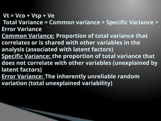
20. Vt = Vco + Vsp + Ve
Total Variance = Common variance + Specific Variance +
Error Variance
Common Variance: Proportion of total variance that
correlates or is shared with other variables in the
analysis (associated with latent factors)
Specific Variance: the proportion of total variance that
does not correlate with other variables (unexplained by
latent factors)
Error Variance: The inherently unreliable random
variation (total unexplained variability)

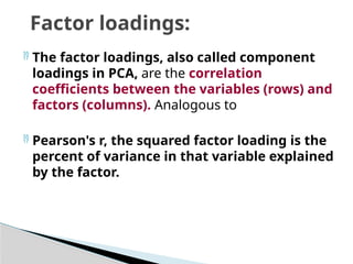
21.  The factor loadings, also called component
loadings in PCA, are the correlation
coefficients between the variables (rows) and
factors (columns). Analogous to
 Pearson's r, the squared factor loading is the
percent of variance in that variable explained
by the factor.
Factor loadings:

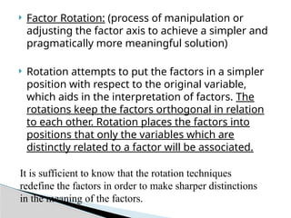
22.  Factor Rotation: (process of manipulation or
adjusting the factor axis to achieve a simpler and
pragmatically more meaningful solution)
 Rotation attempts to put the factors in a simpler
position with respect to the original variable,
which aids in the interpretation of factors. The
rotations keep the factors orthogonal in relation
to each other. Rotation places the factors into
positions that only the variables which are
distinctly related to a factor will be associated.
It is sufficient to know that the rotation techniques
redefine the factors in order to make sharper distinctions
in the meaning of the factors.

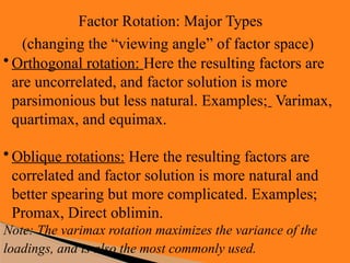
23. Factor Rotation: Major Types
(changing the “viewing angle” of factor space)
• Orthogonal rotation: Here the resulting factors are
are uncorrelated, and factor solution is more
parsimonious but less natural. Examples; Varimax,
quartimax, and equimax.
• Oblique rotations: Here the resulting factors are
correlated and factor solution is more natural and
better spearing but more complicated. Examples;
Promax, Direct oblimin.
Note: The varimax rotation maximizes the variance of the
loadings, and is also the most commonly used.

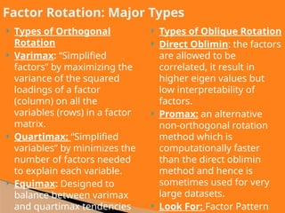
24.  Types of Orthogonal
Rotation
 Varimax: “Simplified
factors” by maximizing the
variance of the squared
loadings of a factor
(column) on all the
variables (rows) in a factor
matrix.
 Quartimax: “Simplified
variables” by minimizes the
number of factors needed
to explain each variable.
 Equimax: Designed to
balance between varimax
and quartimax tendencies
 Types of Oblique Rotation
 Direct Oblimin: the factors
are allowed to be
correlated, it result in
higher eigen values but
low interpretability of
factors.
 Promax: an alternative
non-orthogonal rotation
method which is
computationally faster
than the direct oblimin
method and hence is
sometimes used for very
large datasets.
 Look For: Factor Pattern
Factor Rotation: Major Types

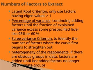
25.  Latent Root Criterion, only use factors
having eigen values > 1
 Percentage of variance, continuing adding
factors until the fraction of explained
variance excess some prespecified level
like 95% or 60 %
 Scree variance Criterion, to identify the
number of factors where the curve first
begins to straighten out
 heterogeneity of the respondents, if there
are obvious groups in data, factors are
added until last added factors no longer
discriminate groups.
Numbers of Factors to Extract

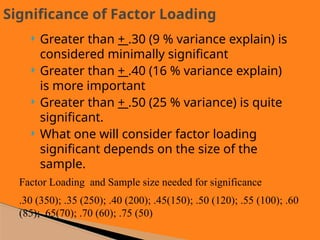
26.  Greater than + .30 (9 % variance explain) is
considered minimally significant
 Greater than + .40 (16 % variance explain)
is more important
 Greater than + .50 (25 % variance) is quite
significant.
 What one will consider factor loading
significant depends on the size of the
sample.
Significance of Factor Loading
Factor Loading and Sample size needed for significance
.30 (350); .35 (250); .40 (200); .45(150); .50 (120); .55 (100); .60
(85); .65(70); .70 (60); .75 (50)

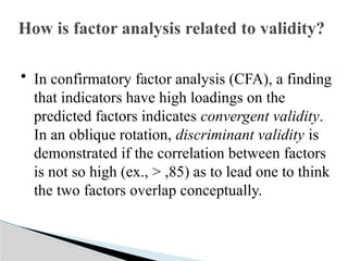
27. How is factor analysis related to validity?
• In confirmatory factor analysis (CFA), a finding
that indicators have high loadings on the
predicted factors indicates convergent validity.
In an oblique rotation, discriminant validity is
demonstrated if the correlation between factors
is not so high (ex., > ,85) as to lead one to think
the two factors overlap conceptually.

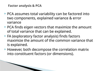
28.  PCA assumes total variability can be factored into
two components, explained variance & error
variance
 PCA finds eigen vectors that maximize the amount
of total variance that can be explained.
 FA (exploratory factor analysis) finds factors
maximize the amount of the common variance that
is explained.
 However, both decompose the correlation matrix
into constituent factors (or dimensions).
Factor analysis & PCA