Downloaded 152 times

![ANOVAb
Model Sum of Squares df Mean Square F Sig.
1 Regression 60.025 3 20.008 4.825 .006a
Residual 157.594 38 4.147
Total 217.619 41
a. Predictors: (Constant), opcontac, age, educ
b. Dependent Variable: monthsfu
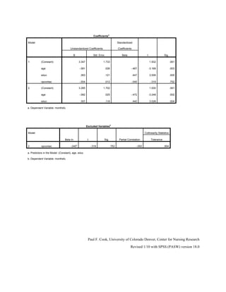
This table gives you an F-test to determine whether the model is a good fit for the data.
According to this p-value, it is.
Coefficientsa
Model
Unstandardized Coefficients
Standardized
Coefficients
t Sig.B Std. Error Beta
1 (Constant) 3.347 1.733 1.932 .061
age -.081 .026 -.467 -3.168 .003
educ .363 .121 .447 3.006 .005
opcontac -.004 .012 -.045 -.319 .752
a. Dependent Variable: monthsfu
Finally, here are the beta coefficients—one to go with each predictor. (Use the “unstandardized
coefficients,” because the constant [beta zero] is included). Based on this table, the equation for
the regression line is:
y = 3.347 - .081(age) + .363(educ) - .004(opcontact)
Using this equation, given values for “age,” “educ,” and “opcontact,” you can come up with a
prediction for the “months of full-time work” variable.](https://image.slidesharecdn.com/multipleregressioninspss-150404045801-conversion-gate01/85/Multiple-regression-in-spss-5-320.jpg)
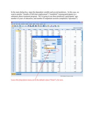
![Now go back to the original dialog box, and change this drop-down menu to use the “stepwise”
method instead.
[For the sake of simplicity, I also went under “statistics” and turned off the “descriptives” option
for the following tests]](https://image.slidesharecdn.com/multipleregressioninspss-150404045801-conversion-gate01/85/Multiple-regression-in-spss-6-320.jpg)


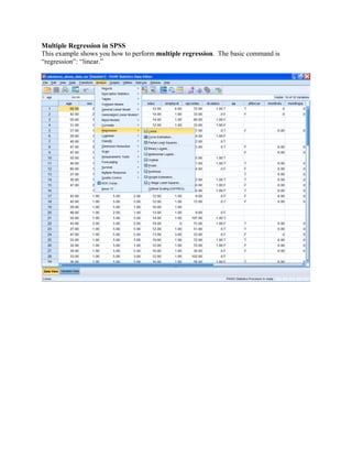
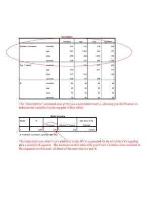
This document provides instructions for performing multiple regression analysis in SPSS. It demonstrates entering variables, running the regression using the enter, stepwise, and backward methods, and interpreting the output including R-square values, F-tests, beta coefficients, and equations for predicting the dependent variable based on the independent variables. Age and education were identified as the best predictors of months of full-time employment using both the stepwise and backward regression methods.