This document discusses efficient algorithms for computing the discrete Fourier transform (DFT), specifically the fast Fourier transform (FFT). It covers several FFT algorithms including decimation-in-time, decimation-in-frequency, and the Goertzel algorithm. The decimation-in-time algorithm recursively breaks down the DFT computation into smaller DFTs by decomposing the input sequence. This allows the computation to be performed in O(NlogN) time rather than O(N^2) time for a direct DFT computation. The document also discusses optimizations like in-place computation to reduce memory usage.

1. Biomedical Signal processing
Chapter 9 Computation of the Discrete
Fourier Transform
Zhongguo Liu
Biomedical Engineering
School of Control Science and Engineering, Shandong
University
02/19/13 1
1 Zhongguo Liu_Biomedical Engineering_Shandong Univ

2. Chapter 9 Computation of the
Discrete Fourier Transform
9.0 Introduction
9.1 Efficient Computation of Discrete Fourier Transform
9.2 The Goertzel Algorithm
9.3 decimation-in-time FFT Algorithms
9.4 decimation-in-frequency FFT Algorithms
9.5 practical considerations （ software realization)
2

3. 9.0 Introduction
Implement a convolution of two sequences
by the following procedure:
1. Compute the N-point DFT X 1 [ k ] and X 2 [ k ]
of the two sequence x1 [ n] and x2 [ n]
2. Compute X 3 [ k ] = X 1 [ k ] X 2 [ k ]for 0 ≤ k ≤ N −1
3. Compute x3 [ n] = x1 [ n] N x2 [ n] the inverse
as
DFT of X 3 [ k ]
Why not convolve the two sequences directly?
There are efficient algorithms called Fast
Fourier Transform (FFT) that can be orders of
3 magnitude more efficient than others.

4. 9.1 Efficient Computation of Discrete
Fourier Transform
The DFT pair was given as
N −1
− j ( 2π / N ) kn 1 N −1
j ( 2π / N ) kn
X [ k ] = ∑ x[n]e x[n] = ∑ X [ k] e
n =0
N k =0
Baseline for computational complexity:
Each DFT coefficient requires
N complex multiplications;
N-1 complex additions
All N DFT coefficients require
N2 complex multiplications;
N(N-1) complex additions
4 4

5. 9.1 Efficient Computation of Discrete
Fourier Transform
N −1
− j ( 2π / N ) kn
X [ k ] = ∑ x[n]e
n =0
Complexity in terms of real operations
4N2 real multiplications
2N(N-1) real additions (approximate 2N2)
5 5

6. 9.1 Efficient Computation of
Discrete Fourier Transform
Most fast methods are based on Periodicity
properties
( Periodicity in n−and /k;) Conjugate )symmetry( 2π / N ) kn
− j 2π / N ) k ( N − n ) j ( 2π N kN − j ( 2π / N k ( − n ) j
e =e e =e
− j ( 2π / N ) kn − j ( 2π / N ) k ( n + N ) j ( 2π / N ) ( k + N ) n
e =e =e
Re { } ]
6 6

7. 9.2 The Goertzel Algorithm
Makes use of the periodicity j ( 2π / N ) Nk
e = e j 2π k = 1
Multiply DFT equation with this factor
j ( 2π / N ) kN
N −1
− j ( 2π / N ) rk N −1
j ( 2π / N ) k ( N −r )
X [ k] = e ∑ x[r ]e = ∑ x[r ]e
r =0 r =0
∞
j ( 2π / N ) k ( n −r )
Define yk [ n ] = ∑ x[r ]e u[ n − r]
r =−∞
using x[n]=0 for n<0 and n>N-1
X [ k ] = yk [ n ] n = N
X[k] can be viewed as the output of a filter to the input x[n]
Impulse response of filter: j ( 2π / N ) kn
h[n] = e u [ n]
X[k] is the output of the filter at time n=N
7 7

8. 9.2 The Goertzel Algorithm
Goertzel j ( 2π / N ) kn
h[n] = e u[n] = W − knu[n]
Filter: N
1
Hk ( z ) =
1 − WN k z −1
−
−
yk [n] = yk [n − 1]WN k + x[n], n = 0,1,..., N , yk [−1] = 0
X [ k ] = yk [ n ] n = N , k = 0,1,..., N
N −1
X [ k ] = ∑ x[n]WN
kn
n =0
Computational complexity
4N real multiplications; 4N real additions
Slightly less efficient than the direct method
But it avoids computation and storage of kn
WN
8 8

9. Second Order Goertzel Filter
Goertzel Filter
1
Hk ( z ) = 2π
j k −1
1− e N z
Multiply both numerator and denominator
− j 2π k −j
2π
k
1− e N
z −1 1− e N
z −1
Hk ( z ) = =
 2π
−1 
− j k −1 
2π 2π k −1 −2
1 − e N z ÷ 1 − e N z ÷ 1 − 2 cos N z + z
j k

  
2π k
y[n] = − y[n − 2] + 2 cos y[n − 1] + x[n], n = 0,1,..., N
N
yk [ N ] = y[ N ] − WNk y[ N − 1] = X [ k ] , k = 0,1, ..., N
9 9

10. Second Order Goertzel Filter
2π k
y[n] = − y[n − 2] + 2 cos y[n − 1] + x[n], n = 0,1,..., N
N
yk [ N ] = y[ N ] − WNk y[ N − 1] = X [ k ] , k = 0,1, ..., N
Complexity for one DFT coefficient ( x(n) is complex
sequence).
Poles: 2N real multiplications and 4N real additions
Zeros: Need to be implement only once:
4 real multiplications and 4 real additions
Complexity for all DFT coefficients
Each pole is used for two DFT coefficients
Approximately N2 real multiplications and 2N2 real
additions
10 10

11. Second Order Goertzel Filter
2π k
y[n] = − y[n − 2] + 2 cos y[n − 1] + x[n], n = 0,1,..., N
N
yk [ N ] = y[ N ] − WNk y[ N − 1] = X [ k ] , k = 0,1, ..., N
If do not need to evaluate all N DFT coefficients
Goertzel Algorithm is more efficient than FFT
if
less than M DFT coefficients are needed,M <
log2N
11 11

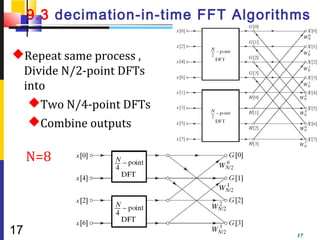
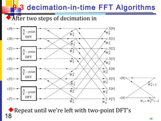
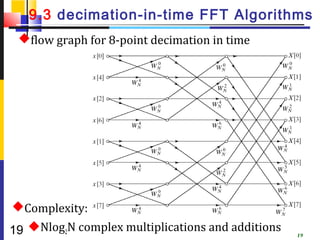
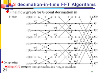
12. 9.3 decimation-in-time FFT Algorithms
Makes use of both periodicity and symmetry
Consider special case of N an integer power of
2
Separate x[n] into two sequence of length N/2
Even indexed samples in the first sequence
Odd indexed samples in the other sequence
N −1
− j ( 2π / N ) kn
X [ k ] = ∑ x[n]e
n =0
− j ( 2π / N ) kn − j ( 2π / N ) kn
= ∑ x[n]e
n even
+ ∑ x[n]e
n odd
12 12

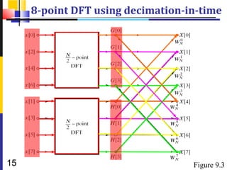
13. 9.3 decimation-in-time FFT Algorithms
− j ( 2π / N ) kn − j ( 2π / N ) kn
X [ k] = ∑ x[n]e + ∑ x[n]e
n even n odd
Substitute variables n=2r for n even and n=2r+1 for odd
N / 2 −1 N / 2 −1
X [ k] = ∑ x[2r ]W 2 rk
N + ∑ x[2r + 1]W ( 2 r +1) k
N
r =0 r =0
N /2 −1 N /2 −1
= ∑
r =0
x[2r ]WN /2 + WN
rk k
∑
r =0
x[2r + 1]WN / 2
rk
= G[ k] +W H [ k] k − j 2π 2 − j 2π
N W 2
N =e N = e N /2 = WN /2
G[k] and H[k] are the N/2-point DFT’s of each subsequence
13 13

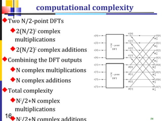
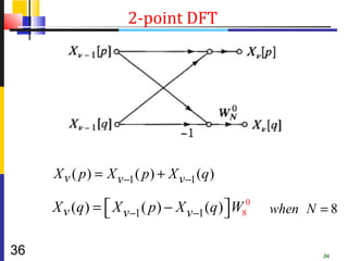
14. 9.3 decimation-in-time FFT Algorithms
N /2 −1 N /2 −1
X [ k] = ∑ x[2r ]W rk
N /2 +W k
N ∑ x[2r + 1]W rk
N /2
r =0 r =0
= G[ k] +W H [ k]k
− j 2π 2 rk − j 2π rk
N
e N = e N /2 = WNrk/2
N −1
k = 0,1,..., k = 0,1,..., N
2
 N  N
G k +  = G [ k ] H k +  = H [ k ]
 2  2
G[k] and H[k] are the N/2-point DFT’s of each subsequence
14 14

15. 8-point DFT using decimation-in-time
15 Figure 9.3

16. computational complexity
Two N/2-point DFTs
2(N/2)2 complex
multiplications
2(N/2)2 complex additions
Combining the DFT outputs
N complex multiplications
N complex additions
Total complexity
N2/2+N complex
multiplications
16 2
 16

17. 9.3 decimation-in-time FFT Algorithms
Repeat same process ,
Divide N/2-point DFTs
into
Two N/4-point DFTs
Combine outputs
N=8
17 17

18. 9.3 decimation-in-time FFT Algorithms
After two steps of decimation in
time
Repeat until we’re left with two-point DFT’s
18 18

19. 9.3 decimation-in-time FFT Algorithms
flow graph for 8-point decimation in time
Complexity:
19 Nlog2N complex multiplications and additions 19

20. Butterfly Computation
Flow graph constitutes of butterflies
We can implement each butterfly with one multiplication
Final complexity for decimation-in-time FFT
(N/2)log2N complex multiplications and additions
20 20

21. 9.3 decimation-in-time FFT Algorithms
Final flow graph for 8-point decimation in
time
Complexity:
(Nlog2N)/2 complex multiplications and Nlog2N additions
21 21

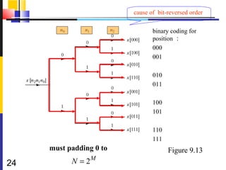
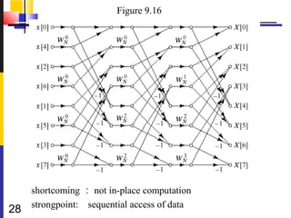
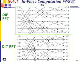
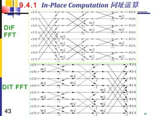
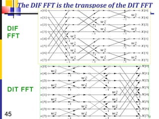
22. 9.3.1 In-Place Computation 同址运
算
Decimation-in-time flow graphs require two sets of
registers
Input and output for each stage
X 0 [ 0] = x [ 0] x [ 0] X 2 [ 0] X [ 0]
X 0 [ 1] = x [ 4] x [ 4] X 2 [ 1] X [ 1]
X 0 [ 2] = x [ 2] x [ 2] X 2 [ 2] X [ 2]
X 0 [ 3] = x [ 6] x [ 6] X 2 [ 3] X [ 3]
X 0 [ 4] = x [ 1] x [ 1] X 2 [ 4] X [ 4]
X 0 [ 5] = x [ 5 ] x [ 5] X 2 [ 5] X [ 5]
X 0 [ 6] = x [ 3] x [ 3] X 2 [ 6] X [ 6]
22X 0 [ 7] = x [ 7] x [ 7] X 2 [ 7] X [ 7] 22

23. 9.3.1 In-Place Computation 同址运 算
Note the arrangement of the input indices
Bit reversed indexing （码位倒置）
X 0 [ 0] = x [ 0] ↔ X 0 [ 000] = x [ 000] x [ 0] X [ 0]
X 0 [ 1] = x [ 4] ↔ X 0 [ 001] = x [ 100] x [ 4] X [ 1]
X 0 [ 2] = x [ 2] ↔ X 0 [ 010] = x [ 010] x [ 2] X [ 2]
X 0 [ 3] = x [ 6] ↔ X 0 [ 011] = x [ 110] x [ 6] X [ 3]
X 0 [ 4] = x [ 1] ↔ X 0 [ 100] = x [ 001] x [ 1] X [ 4]
X 0 [ 5] = x [ 5] ↔ X 0 [ 101] = x [ 101] x [ 5] X [ 5]
X 0 [ 6] = x [ 3] ↔ X 0 [ 110] = x [ 011] x [ 3] X [ 6]
X 0 [ 7 ] = x [ 7 ] ↔ X 0 [ 111] = x [ 111] x [ 7] X [ 7]
23 23

24. cause of bit-reversed order
binary coding for
position ：
000
001
010
011
100
101
110
111
must padding 0 to Figure 9.13
24 N = 2M

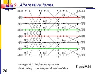
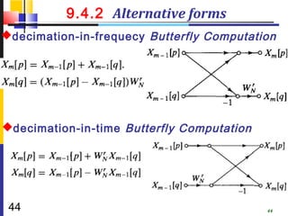
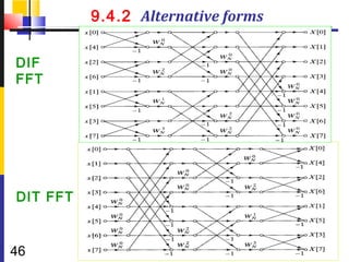
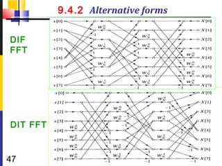
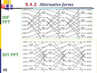
25. 9.3.2 Alternative forms
Note the arrangement of the input indices
Bit reversed indexing （码位倒置）
X 0 [ 0] = x [ 0] ↔ X 0 [ 000] = x [ 000] x [ 0] X [ 0]
X 0 [ 1] = x [ 4] ↔ X 0 [ 001] = x [ 100] x [ 4] X [ 1]
X 0 [ 2] = x [ 2] ↔ X 0 [ 010] = x [ 010] x [ 2] X [ 2]
X 0 [ 3] = x [ 6] ↔ X 0 [ 011] = x [ 110] x [ 6] X [ 3]
X 0 [ 4] = x [ 1] ↔ X 0 [ 100] = x [ 001] x [ 1] X [ 4]
X 0 [ 5] = x [ 5] ↔ X 0 [ 101] = x [ 101] x [ 5] X [ 5]
X 0 [ 6] = x [ 3] ↔ X 0 [ 110] = x [ 011] x [ 3] X [ 6]
X 0 [ 7 ] = x [ 7 ] ↔ X 0 [ 111] = x [ 111] x [ 7] X [ 7]
25 25

26. 9.3.2 Alternative forms
strongpoint ： in-place computations
shortcoming ： non-sequential access of data
Figure 9.14
26

27. Figure 9.15
shortcoming ： not in-place computation
non-sequential access of data
27

28. Figure 9.16
shortcoming ： not in-place computation
strongpoint: sequential access of data
28

29. 9.3 decimation-in-time FFT Algorithms
− j ( 2π / N ) kn − j ( 2π / N ) kn
X [ k] = ∑ x[n]e + ∑ x[n]e
n even n odd
Substitute variables n=2r for n even and n=2r+1 for odd
N / 2 −1 N / 2 −1
X [ k] = ∑ x[2r ]W 2 rk
N + ∑ x[2r + 1]W ( 2 r +1) k
N
r =0 r =0
Review
N /2 −1 N /2 −1
= ∑
r =0
x[2r ]WN /2 + WN
rk k
∑
r =0
x[2r + 1]WN / 2
rk
= G[ k] +W H [ k] k − j 2π 2 − j 2π
N W 2
N =e N = e N /2 = WN /2
G[k] and H[k] are the N/2-point DFT’s of each subsequence
29 29

30. 9.3.1 In-Place Computation 同址运 算
Bit reversed indexing （码位倒置）
X 0 [ 000] = x [ 000] x [ 0] X [ 0]
X 0 [ 001] = x [ 100] x [ 4] X [ 1]
X 0 [ 010] = x [ 010] x [ 2] X [ 2]
X 0 [ 011] = x [ 110] x [ 6] X [ 3]
X 0 [ 100] = x [ 001] x [ 1] X [ 4]
X 0 [ 101] = x [ 101] x [ 5] X [ 5]
X 0 [ 110] = x [ 011] x [ 3] X [ 6]
X 0 [ 111] = x [ 111] x [ 7] X [ 7]
30 30

31. 9.3.2 Alternative forms
strongpoint ： in-place computations
shortcoming ： non-sequential access of data
Figure 9.14
31

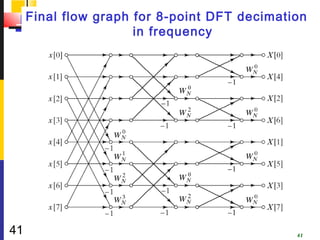
32. 9.4 Decimation-In-Frequency FFT Algorithm
N −1
The DFT equation X [ k ] = ∑ x[n]WN
nk
n =0
Split the DFT equation into even and odd frequency indexes
N −1 N / 2 −1 N −1
X [ 2r ] = ∑ x[n]WN 2 r =
n
∑ x[n]WN 2 r +
n
∑ x[n]WN 2 r
n
n =0 n =0 n= N / 2
N /2 −1 N / 2 −1
Substitute
variables
= ∑ x[n]W
n =0
n2r
N + ∑ x[n + N / 2]W
n =0
( n + N /2 ) 2 r
N
N / 2 −1
= ∑ ( x[n] + x[n + N / 2]) W
n =0
nr
N /2
N /2 −1
= ∑ rn
g (n)WN / 2
32 n =0
32

33. 9.4 Decimation-In-Frequency FFT Algorithm
N −1
The DFT equation X [ k ] = ∑ x[n]WN
nk
n =0
N −1 N /2 −1 N −1
X [ 2r + 1] = ∑ x[n]W n (2 r +1)
N = ∑ x[n]W n (2 r +1)
N + ∑ x[n]W n (2 r +1)
N
n=0 n=0 n = N /2
N /2 −1 N /2 −1
= ∑
n =0
x[n]W n (2 r +1)
N + ∑ x[n + N / 2]W
n =0
N
( n + N / 2 ) (2 r +1)
N /2 −1
= ∑ ( x[n] − x[n + N / 2]) W
n =0
n (2 r +1)
N
N / 2 −1 N /2 −1
= ∑ ( x[n] − x[n + N / 2]) W W n
N
rn
N /2
= ∑n =0
h(n)WN WNn2
n r
/
n =0
N
n ( 2 r +1) (2 r +1)
W N =W W =W W
2 rn
N
n
N
rn
N /2
n
N W 2
= WNNrWNN / 2 = −1
33 N
33

34. decimation-in-frequency decomposition of an N-
point DFT to N/2-point DFT
N /2 −1 N /2 −1
X [ 2r ] = ∑ ( x[n] + x[n + N / 2]) WN /2=
nr
∑ rn
g (n)WN /2
n = 0 /2 −1
N n =0 N /2 −1
X [ 2r + 1] =
34 ∑
n =0
( x[n] − x[n + N / 2]) WN W
n rn
N /2
= ∑
n =0
h(n)WN WNn2
n r
34
/

35. decimation-in-frequency decomposition of an 8-
point DFT to four 2-point DFT
N / 4 −1 N / 4 −1
X [ 2* 2 s ] = ∑ [ g (n) + g (n + N / 4)]WNsn =
/4 ∑ p(n)WNsn
/4
n =0 n =0
N / 4 −1 N /4 −1
X [ 2*(2 s + 1) ] = ∑ [ g (n) − g (n + N / 4)]W W
2n sn
= ∑ q ( n)WN nWNn
2 s
35 n =0
N N /4
n =0 35
/4

36. 2-point DFT
X v ( p ) = X v−1 ( p ) + X v −1 (q )
X v (q ) =  X v −1 ( p ) − X v−1 (q )  W80
  when N = 8
36 36

37. N /2 −1 N /2 −1
X [ 2r ] = ∑ ( x[n] + x[n + N / 2]) nr
WN /2 = ∑ rn
g (n)WN /2
n =0 n =0
N /4 −1 N /2 −1
X [ 2* 2 s ] = ∑ g (n)WN /2 +
2 sn
∑ 2 sn
g (n)WN /2
n =0 n = N /4
N /4 −1 N /4 −1
= ∑
n =0
g (n)WN /2 +
2 sn
∑
n =0
g (n + N / 4)WN /2( n + N /4)
2s
N /4 −1 N /4 −1
= ∑ g (n)W
n =0
sn
N /4 + ∑ g (n + N / 4)W
n =0
sn
N /4
N /4 −1 N /4 −1
= ∑ [ g (n) + g (n + N / 4)]W sn
N /4
= ∑
n =0
p(n)WNsn
/4
n =0
37

38. N /2 −1 N /2 −1
X [ 2r ] = ∑ ( x[n] + x[n + N / 2]) nr
WN /2 = ∑ rn
g (n)WN /2
n =0 n =0
N /2 −1
X [ 2*(2 s + 1) ] = ∑ g (n)WN /2 +1) n
(2 s
n =0
N /4 −1 N /2 −1
= ∑
n =0
g (n)WN /2+1) n +
(2 s
∑
n= N / 4
g (n)WN /2 +1) n
(2 s
N /4 −1 N /4 −1
= ∑
n =0
g (n)WNsn WN /2 +
/4
n
∑
n =0
g (n + N / 4)WN /2+1)( n + N /4)
(2 s
N /4 −1 N /4 −1
= ∑
n =0
g (n)WNsn WN n +
/4
2
∑
n =0
g (n + N / 4)WNsn WN nWN / 2+1) N /4
/4
2 (2 s
N /4 −1 N /4 −1
= ∑ [ g (n) − g (n + N / 4)]W 2n
N W sn
N /4
= ∑
n =0
q (n)WN nWNsn
2
/4
n =0
38 WN /2 +1) N /4 = WNsN /2WNN/2 = −1
(2 s
/2
/4

39. N /4 −1
X [ 2* 2 s ] = ∑ p (n)WNsn
/4
n =0
N /4 −1
X [ 2* 2* 2t ] = ∑ p (n)W 2 tn
N /4
n =0
N /8 −1 N /4 −1
= ∑
n =0
p (n)W 2 tn
N /4 + ∑
n = N /8
p (n)W 2 tn
N /4
N /8 −1 N /8 −1
= ∑n =0
p (n)W 2 tn
N /4 + ∑
n =0
p(n + N / 8)W 2 t ( n + N /8)
N /4
N /8 −1
= ∑ n =0
[ p(n) + p (n + N / 8)]WN /8
tn
= p(n) + p (n + 1) when N = 8
39

40. N /4 −1
X [ 2* 2 s ] = ∑ p (n)WNsn
/4
n =0
N /4 −1
X [ 2* 2*(2t + 1) ] = ∑ p(n)WN /4+1) n
(2 t
n =0
N /8 −1 N /4 −1
= ∑n =0
p (n)WN /4+1) n +
(2 t
∑
n = N /8
p (n)WN / 4+1) n
(2 t
N /8 −1 N /8 −1
= ∑n =0
p (n)WN /4+1) n +
(2 t
∑
n =0
p (n + N / 8)WN /4+1)( n + N /8)
(2 t
N /8 −1 N /8−1
= ∑
n =0
p (n)WN /4WN /4 +
2 tn n
∑
n =0
p (n + N / 8)WN /4WN /4WN /4+1) N /8
2 tn n (2 t
N /8 −1
= ∑ [ p(n) − p(n + N / 8)]WN /8WN n
tn 4
n =0 WN(2/4+1) N /8 = WNtN /4WNN/4 = − 1
t
/4
/8
= [ p (n) − p (n + 1)]W80 when N = 8
40

41. Final flow graph for 8-point DFT decimation
in frequency
41 41

42. 9.4.1 In-Place Computation 同址运
算
DIF
FFT
DIT FFT
42 42

43. 9.4.1 In-Place Computation 同址运 算
DIF
FFT
DIT FFT
43 43

44. 9.4.2 Alternative forms
decimation-in-frequecy Butterfly Computation
decimation-in-time Butterfly Computation
44 44

45. The DIF FFT is the transpose of the DIT FFT
DIF
FFT
DIT FFT
45 45

46. 9.4.2 Alternative forms
DIF
FFT
DIT FFT
46

47. 9.4.2 Alternative forms
DIF
FFT
DIT FFT
47

48. Figure 9.24 erratum
x [ 0]
x [ 4]
x [ 2]
x [ 6]
x [ 1]
x [ 5]
x [ 3]
x [ 7]
48

49. 9.4.2 Alternative forms
DIF
FFT
DIT FFT
49

50. Chapter 9 HW
9.1, 9.2, 9.3,
50
50 返 回02/19/13 上一页
Zhongguo Liu_Biomedical Engineering_Shandong
下一页 Univ.