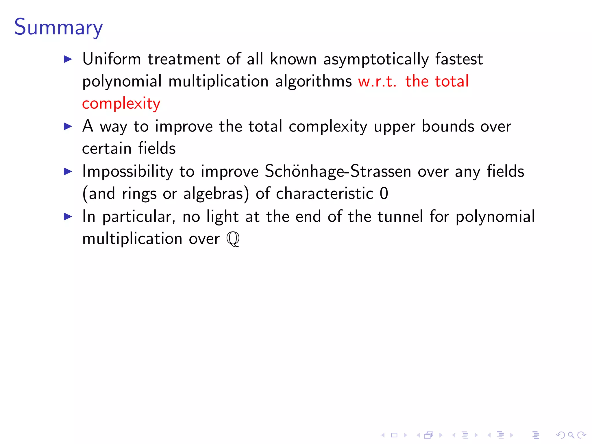
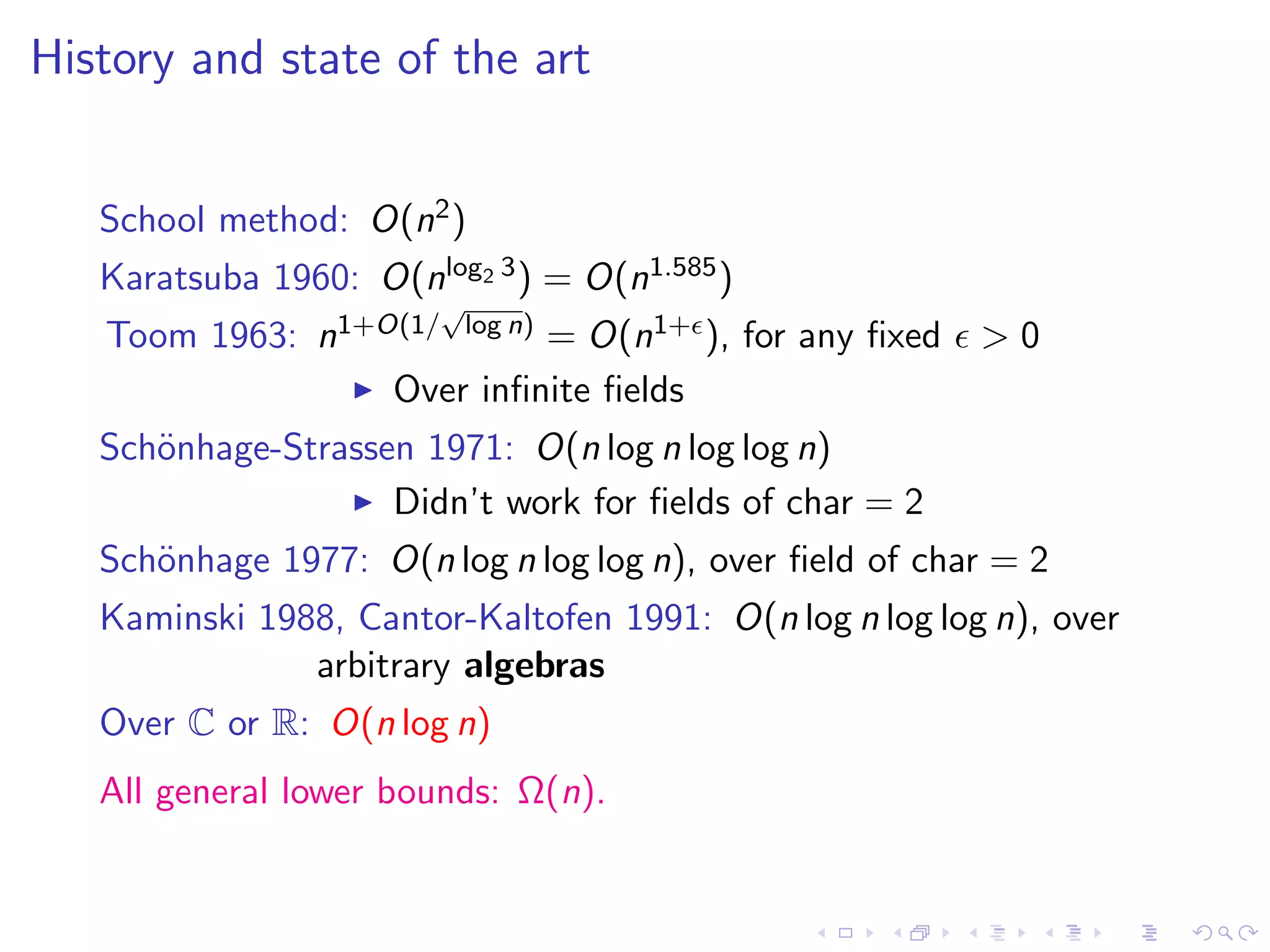
This document discusses faster algorithms for polynomial multiplication via discrete Fourier transforms (DFTs). It summarizes the history of polynomial multiplication algorithms, including approaches with complexity O(n^1.585), O(n log n log log n), and O(n log n). The document proposes a framework for analyzing polynomial multiplication algorithms based on attaching roots of unity via algebraic field extensions and performing DFTs and IDFTs over the extensions. This approach relates the complexity to properties of the degree function of the base field. Fields with degree functions growing slowly allow faster algorithms, while fields like the rationals require different approaches due to a lower complexity bound of Ω(n log n log log n).

1. Faster Polynomial Multiplication via
Discrete Fourier Transforms
Alexey Pospelov
Computer Science Department, Saarland University
Cluster of Excellence Multimodal Computing and Interaction
June 14th, 2011

2. Polynomial multiplication
Given
a(x) = a0 + a1 x + · · · + an x n , b(x) = b0 + b1 x + · · · + bn x n ,
Compute
c(x) = c0 + c1 x + · · · + c2n x 2n = a(x)b(x).

3. Polynomial multiplication
Given
a(x) = a0 + a1 x + · · · + an x n , b(x) = b0 + b1 x + · · · + bn x n ,
Compute
c(x) = c0 + c1 x + · · · + c2n x 2n = a(x)b(x).
For all 0 ≤ i ≤ 2n, compute
a0 bi + a1 bi−1 + · · · + ai b0 , 0 ≤ i ≤ n,
ci =
ai−n bn + ai−n+1 bn−1 + · · · + an bi−n , n < i ≤ 2n.

4. In what model?
Arithmetic circuits with binary “+”, “−”, “·”
Each binary gate has unit cost
No divisions
Constants from the field available at no cost
Inputs are the coefficients of the polynomials to be multiplied
Outputs are the coefficients of the product polynomial
Interested in a circuit for degree n polynomial multiplication
of the minimal size

5. History and state of the art
School method: O(n2 )
Karatsuba 1960: O(nlog2 3 ) = O(n1.585 )
√
Toom 1963: n1+O(1/ log n) = O(n1+ ), for any fixed >0
Over infinite fields

6. History and state of the art
School method: O(n2 )
Karatsuba 1960: O(nlog2 3 ) = O(n1.585 )
√
Toom 1963: n1+O(1/ log n) = O(n1+ ), for any fixed >0
Over infinite fields
Sch¨nhage-Strassen 1971: O(n log n log log n)
o
Didn’t work for fields of char = 2

7. History and state of the art
School method: O(n2 )
Karatsuba 1960: O(nlog2 3 ) = O(n1.585 )
√
Toom 1963: n1+O(1/ log n) = O(n1+ ), for any fixed >0
Over infinite fields
Sch¨nhage-Strassen 1971: O(n log n log log n)
o
Didn’t work for fields of char = 2
Sch¨nhage 1977: O(n log n log log n), over field of char = 2
o
Kaminski 1988, Cantor-Kaltofen 1991: O(n log n log log n), over
arbitrary algebras
Over C or R: O(n log n)
All general lower bounds: Ω(n).

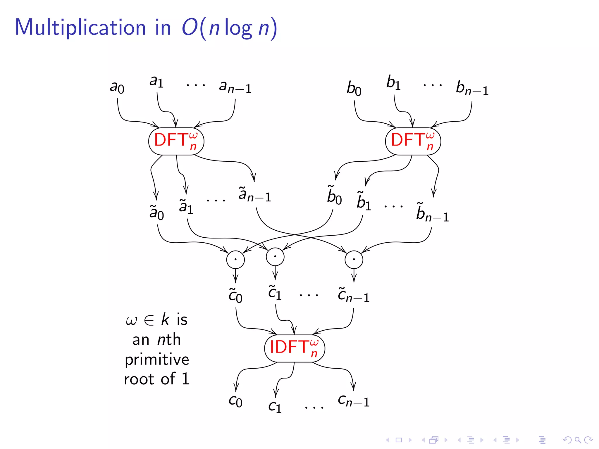
8. Multiplication in O(n log n)
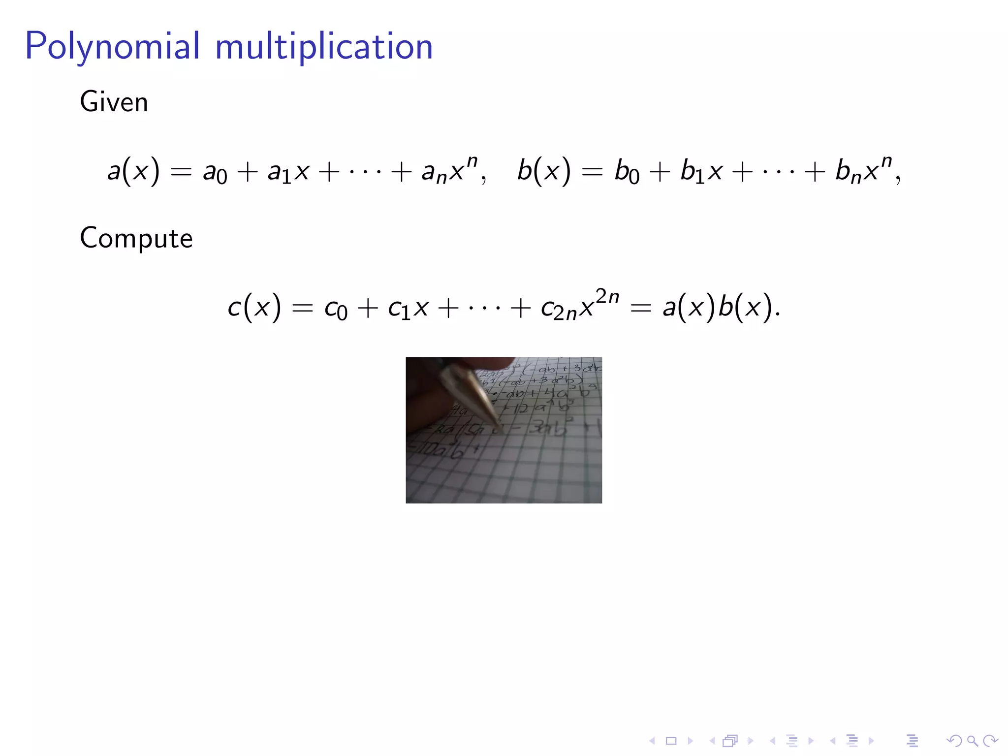
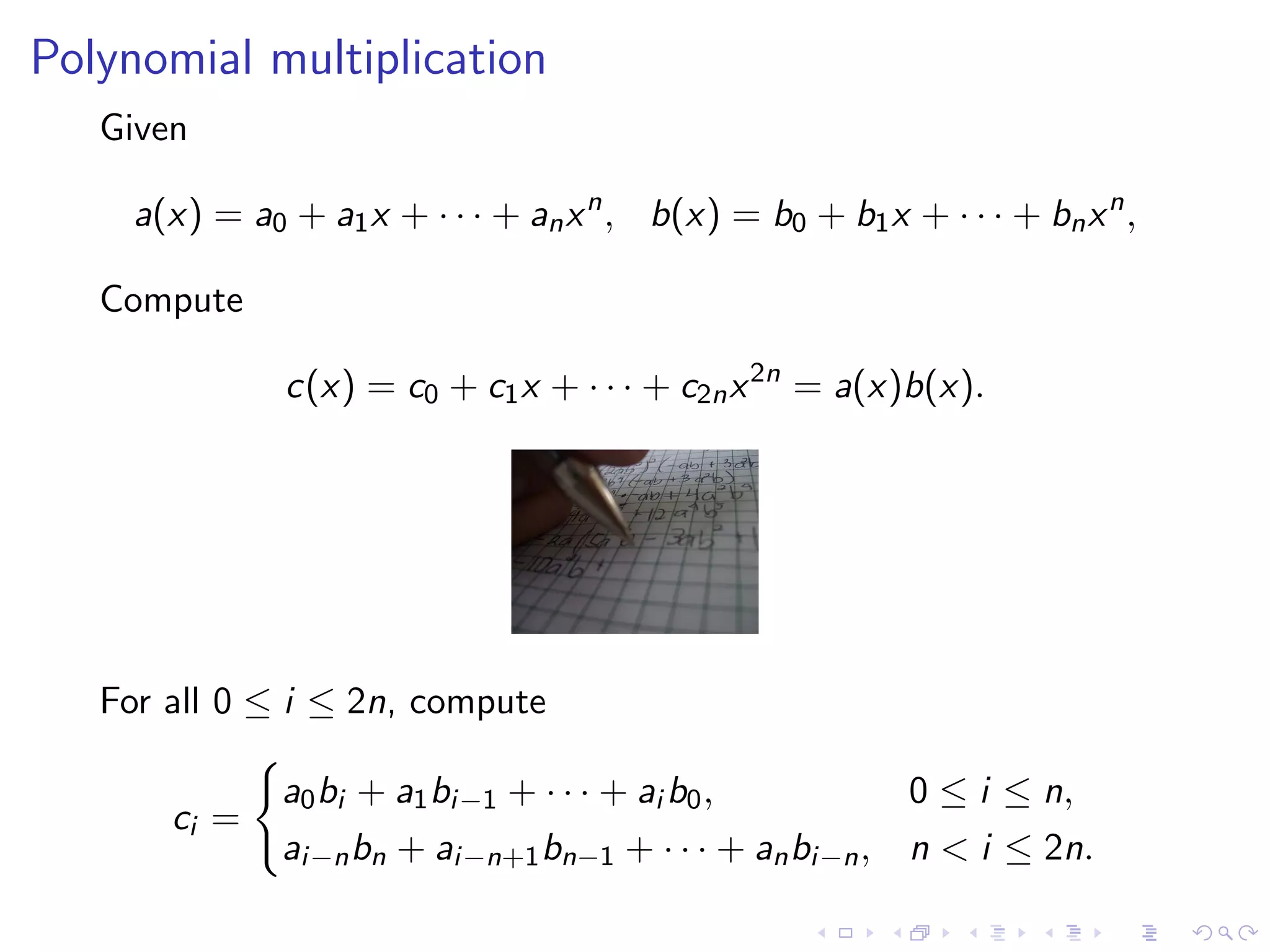
Given
a(x) = a0 + a1 x + · · · + an−1 x n−1 ,
b(x) = b0 + b1 x + · · · + bn−1 x n−1 ,
Compute
c(x) = c0 + c1 x + · · · + xn−1 x n−1 = a(x)b(x) (mod x n − 1).
(Can always choose a larger n and pad polynomials with zeroes to
reduce the ordinary polynomial multiplication to the product in
k[x]/(x n − 1).)

9. Multiplication in O(n log n)
a0 a1 . . . an−1 b0 b1 . . . bn−1
8 x 8 x
DFTω
n DFTω
n
. . . ˜n−1
a ˜ ˜
b0 b1 . . .
˜0 ˜1
a a ˜n−1
b
5 { 5 { 5 {
· · ·
c0
˜ c1 . . . cn−1
˜ ˜
ω ∈ k is
8 x
an nth IDFTω
n
primitive
root of 1
c0 c1 . . . cn−1

10. Discrete Fourier transform

11. Discrete Fourier transform
Maps a degree n − 1 polynomial to its values at n distinct nth
roots of unity:
n−1
˜i := a(ω i ) =
a aj ω ij , 0≤i ≤n−1
j=0
DFTω : (a0 , a1 , . . . , an−1 ) → (˜0 , ˜1 , . . . , ˜n−1 )
n a a a
(ω is a primitive nth root of unity)
Linear transform: DFTω : k[x] → k n
n
Isomorphism: DFTω : k[x]/(x n − 1) → k n
n
Can be often computed in O(n log n)
The inverse isomorphism is almost a DFT again:
1 n−1
DFTω
n : (˜0 , ˜1 , . . . , ˜n−1 ) → (a0 , a1 , . . . , an−1 )
a a a
n

12. Discrete Fourier transform
a0 a1 . . . an−1 b0 b1 . . . bn−1
8 x 8 x
DFTω
n DFTω
n
. . . ˜n−1
a ˜ ˜
b0 b1 . . .
˜0 ˜1
a a ˜n−1
b
5 { 5 { 5 {
· · ·
c0
˜ c1 . . . cn−1
˜ ˜
ω ∈ k is
8 x
an nth IDFTω
n
primitive
root of 1
c0 c1 . . . cn−1

13. Discrete Fourier transform
Lk (n): the complexity of degree n polynomial multiplication
over a field k
Dk (n): the complexity of computing length n DFT over k
Lk (n) ≤ 3Dk (n) + 2n = O(n log n).
Note: we need roots of unity.

14. What if roots of unity are not available?

15. What if roots of unity are not available?
Attach them!

16. What if roots of unity are not available?
Attach them!
Switch from the field k to its algebraic extension Am where
roots of unity of sufficiently large order exist.

17. What if roots of unity are not available?
Attach them!
Switch from the field k to its algebraic extension Am where
roots of unity of sufficiently large order exist.
More precisely: take a (ring) extension Am of k of degree m
over k with a 2 th root of unity ω ∈ Am :
For example,
Am = k[x]/pm (x),
pm (x) ∈ k[x] is a polynomial of degree m,
pm (x) vanishes on ω2 ,
(ω2 is a primitive 2 th root of unity in the algebraic closure of
the field k.)

18. What if roots of unity are not available?
Attach them!
Switch from the field k to its algebraic extension Am where
roots of unity of sufficiently large order exist.
More precisely: take a (ring) extension Am of k of degree m
over k with a 2 th root of unity ω ∈ Am :
For example,
Am = k[x]/pm (x),
pm (x) ∈ k[x] is a polynomial of degree m,
pm (x) vanishes on ω2 ,
(ω2 is a primitive 2 th root of unity in the algebraic closure of
the field k.)
How can it help?

19. What if roots of unity are not available?
Attach them!
Switch from the field k to its algebraic extension Am where
roots of unity of sufficiently large order exist.
More precisely: take a (ring) extension Am of k of degree m
over k with a 2 th root of unity ω ∈ Am :
For example,
Am = k[x]/pm (x),
pm (x) ∈ k[x] is a polynomial of degree m,
pm (x) vanishes on ω2 ,
(ω2 is a primitive 2 th root of unity in the algebraic closure of
the field k.)
How can it help? See next slide.

20. Fast polynomial multiplication
a0 . . . a m −1 . . . an−1
2 b0 . . . b m −1 . . . bn−1
2
% } % % } %
→ Am ... → Am → Am ... → Am
A0 7 y A2 −1 B0 7 y B2 −1
DFTω
2 DFTω
2
˜
A2 −1 ˜
B0
˜
A0 5 y 7 { B2
˜
· ... · −1
2 ·m =n ˜
C0 7 y ˜
C2 −1
Am = k[x]/pm (x) IDFTω
2
C0 C2 −1
ω ∈ Am
is a 2 th
primitive ← Am ... ← Am
root of 1 Õ 3 Ù
c0 . . . cm−1 . . . cn−1

21. Fast polynomial multiplication
In this case
Lk (n) ≤ 2 Lk (m)
+ 3DAm (n) · complexity of aritrhmetics in Am
+ cost of embedding and unembedding in Am
Our contribution #1:
Formalize this kind of algorithms
The relation between m and 2 is a barrier for the algorithm’s
performance
This relation depends heavily on the field properties
The cost of the DFT can usually be made O(n log n)
Embedding and unembedding run usually in linear time, e.g.,
if pm (x) is sparse

22. Does it work?
Yes!!!
Sch¨nhage-Strassen 1971:
o =m
Sch¨nhage 1977: 3 = 2m (+ a little trick)
o
Kaminski 1988: = φ(m) (Euler’s totient function)
Cantor-Kaltofen 1991: = m (and Am is a little more complicated
than k[x]/pm (x))

23. Slow fields

24. Slow fields
Recall:
Lk (n) ≤ 2 Lk (m)
+ 3DAm (n) · complexity of arithmetics in Am
+ cost of embedding and unembedding in Am
Ideally we want m to be small and to be large.

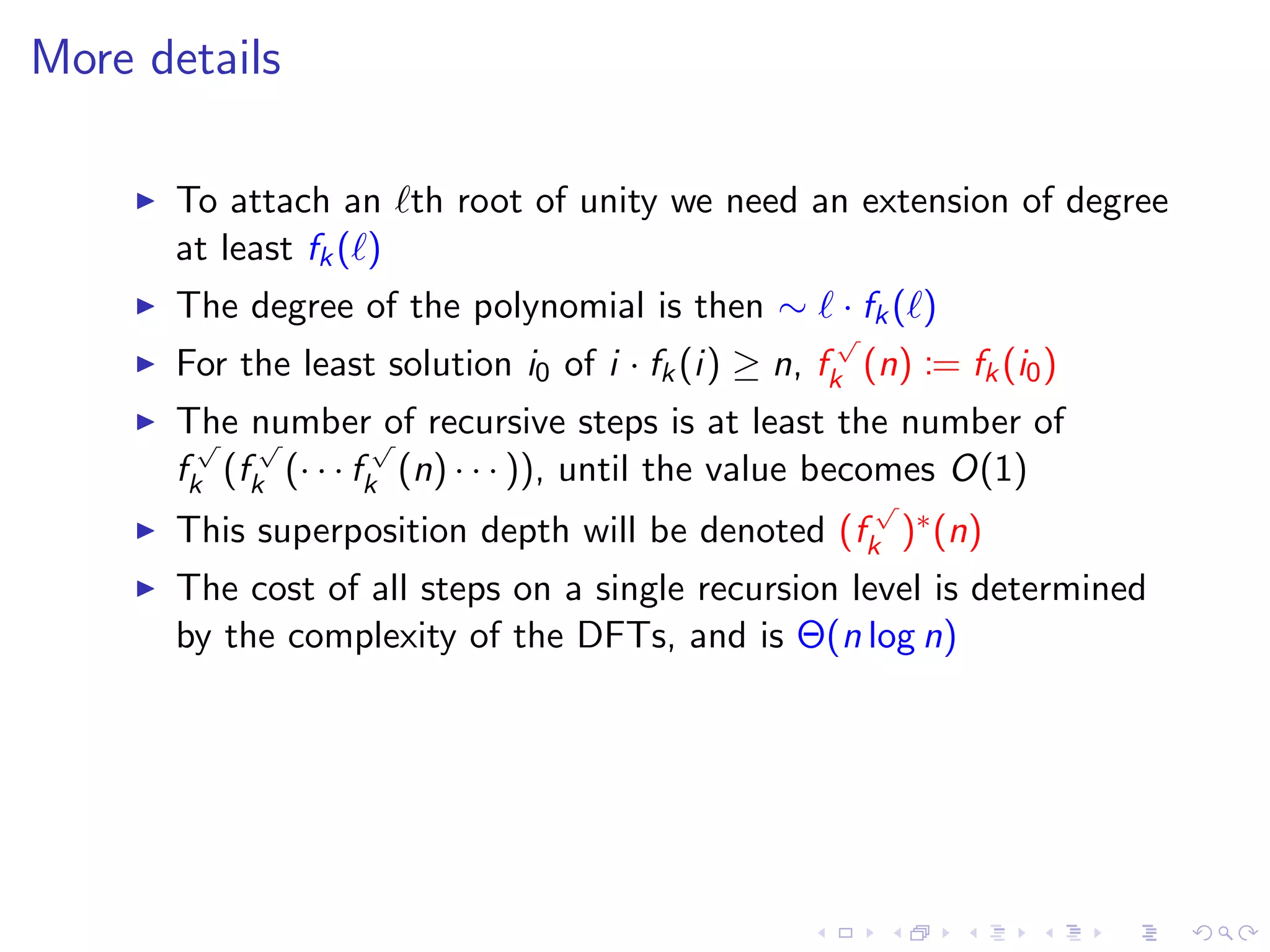
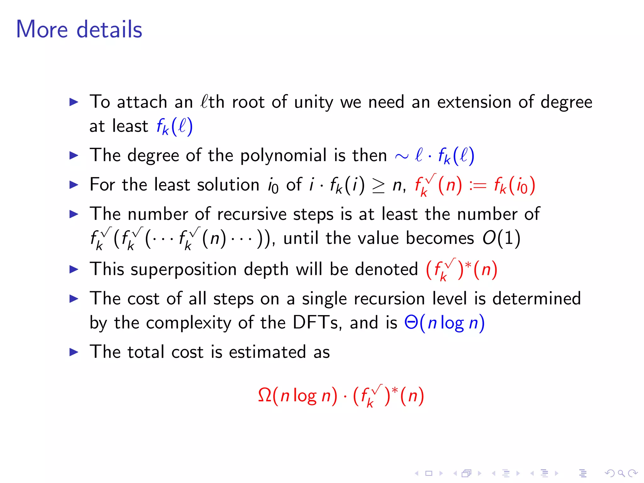
25. Slow fields
Recall:
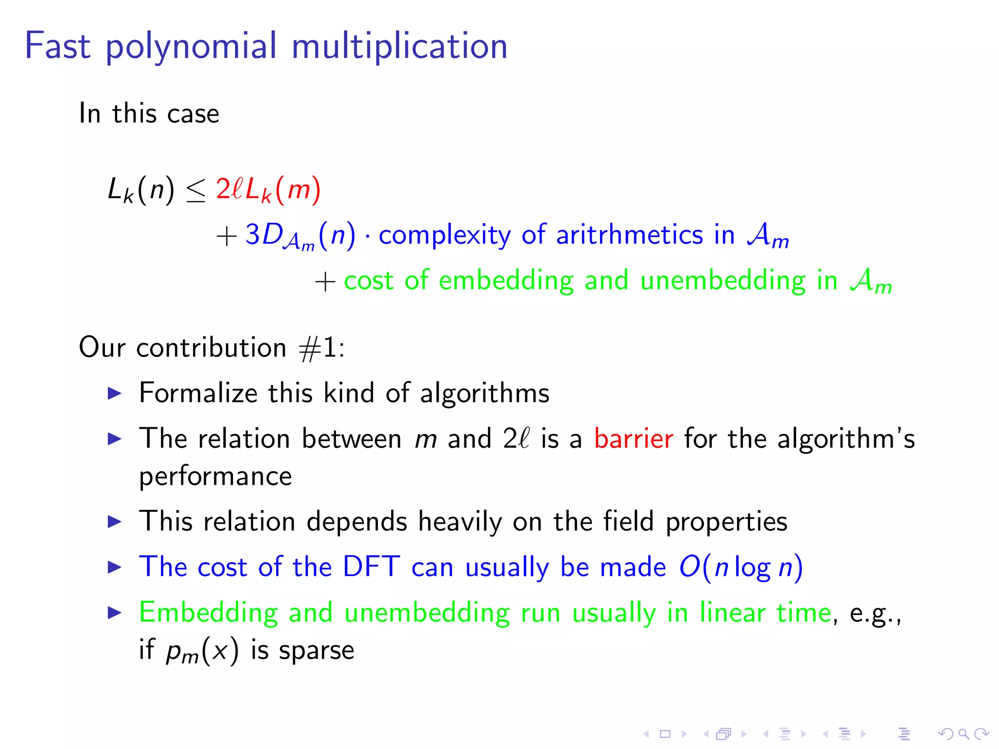
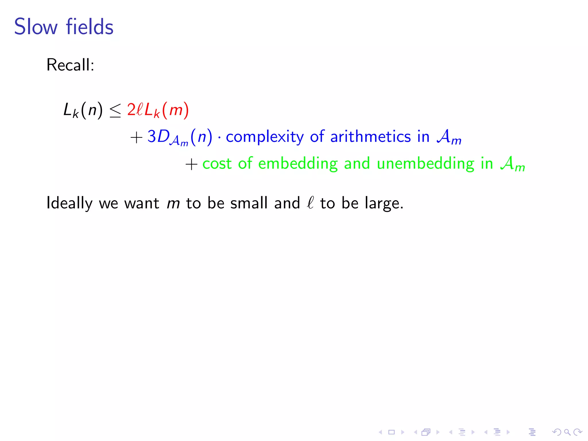
Lk (n) ≤ 2 Lk (m)
+ 3DAm (n) · complexity of arithmetics in Am
+ cost of embedding and unembedding in Am
Ideally we want m to be small and to be large.
Definition
For a field k, and n, s.t. char k n, let fk (n) be [k(ωn ) : k], the
degree function of k.

26. Slow fields
Recall:
Lk (n) ≤ 2 Lk (m)
+ 3DAm (n) · complexity of arithmetics in Am
+ cost of embedding and unembedding in Am
Ideally we want m to be small and to be large.
Definition
For a field k, and n, s.t. char k n, let fk (n) be [k(ωn ) : k], the
degree function of k.
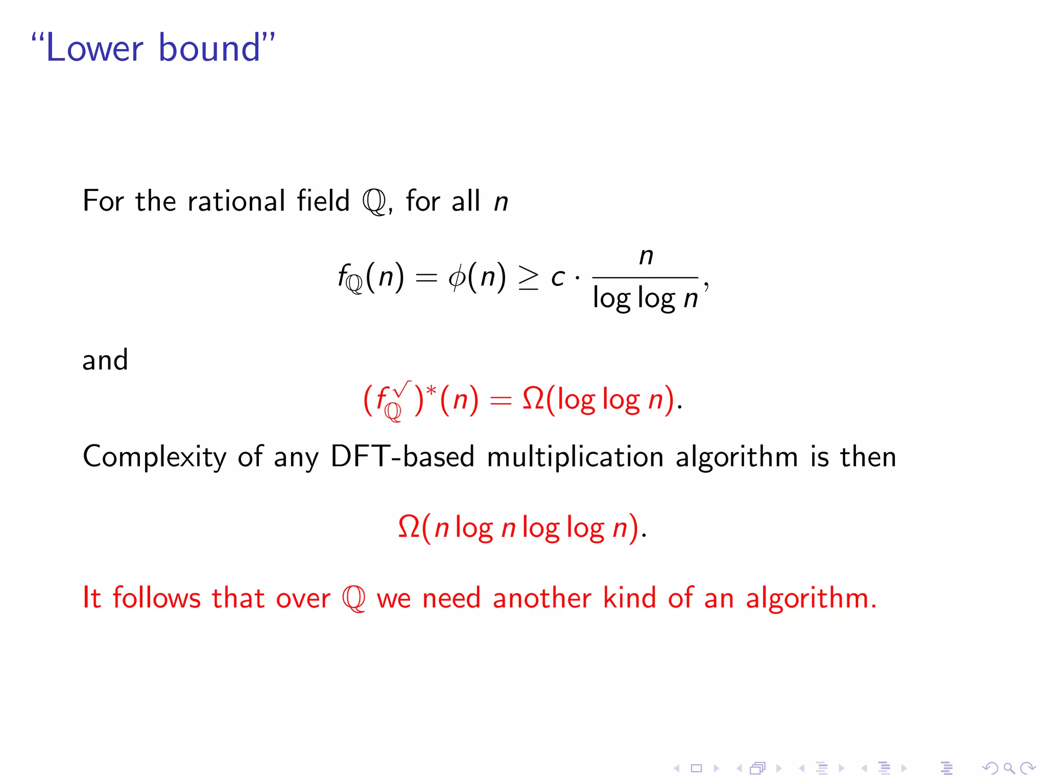
Our contribution #2:
If fk (n) = o(log log n) for some not too sparse set of n then k
is fast and Lk (n) = o(n log n log log n)
If fk (n) = Ω(n1− ) for any fixed 0, then k is slow and any
algorithm of that kind runs in Ω(n log n log log n)

27. More details
To attach an th root of unity we need an extension of degree
at least fk ( )
The degree of the polynomial is then ∼ · fk ( )
√
For the least solution i0 of i · fk (i) ≥ n, fk (n) := fk (i0 )
The number√of recursive steps is at least the number of
√ √
fk (fk (· · · fk (n) · · · )), until the value becomes O(1)
√
This superposition depth will be denoted (fk )∗ (n)
The cost of all steps on a single recursion level is determined
by the complexity of the DFTs, and is Θ(n log n)

28. More details
To attach an th root of unity we need an extension of degree
at least fk ( )
The degree of the polynomial is then ∼ · fk ( )
√
For the least solution i0 of i · fk (i) ≥ n, fk (n) := fk (i0 )
The number√of recursive steps is at least the number of
√ √
fk (fk (· · · fk (n) · · · )), until the value becomes O(1)
√
This superposition depth will be denoted (fk )∗ (n)
The cost of all steps on a single recursion level is determined
by the complexity of the DFTs, and is Θ(n log n)
The total cost is estimated as
√
Ω(n log n) · (fk )∗ (n)

29. “Lower bound”
For the rational field Q, for all n
n
fQ (n) = φ(n) ≥ c · ,
log log n
and √
(fQ )∗ (n) = Ω(log log n).

30. “Lower bound”
For the rational field Q, for all n
n
fQ (n) = φ(n) ≥ c · ,
log log n
and √
(fQ )∗ (n) = Ω(log log n).
Complexity of any DFT-based multiplication algorithm is then
Ω(n log n log log n).
It follows that over Q we need another kind of an algorithm.

31. Summary
Uniform treatment of all known asymptotically fastest
polynomial multiplication algorithms w.r.t. the total
complexity
A way to improve the total complexity upper bounds over
certain fields
Impossibility to improve Sch¨nhage-Strassen over any fields
o
(and rings or algebras) of characteristic 0
In particular, no light at the end of the tunnel for polynomial
multiplication over Q

32. Summary
Uniform treatment of all known asymptotically fastest
polynomial multiplication algorithms w.r.t. the total
complexity
A way to improve the total complexity upper bounds over
certain fields
Impossibility to improve Sch¨nhage-Strassen over any fields
o
(and rings or algebras) of characteristic 0
In particular, no light at the end of the tunnel for polynomial
multiplication over Q
Over fields of positive characteristic,

33. Thank you for attention!