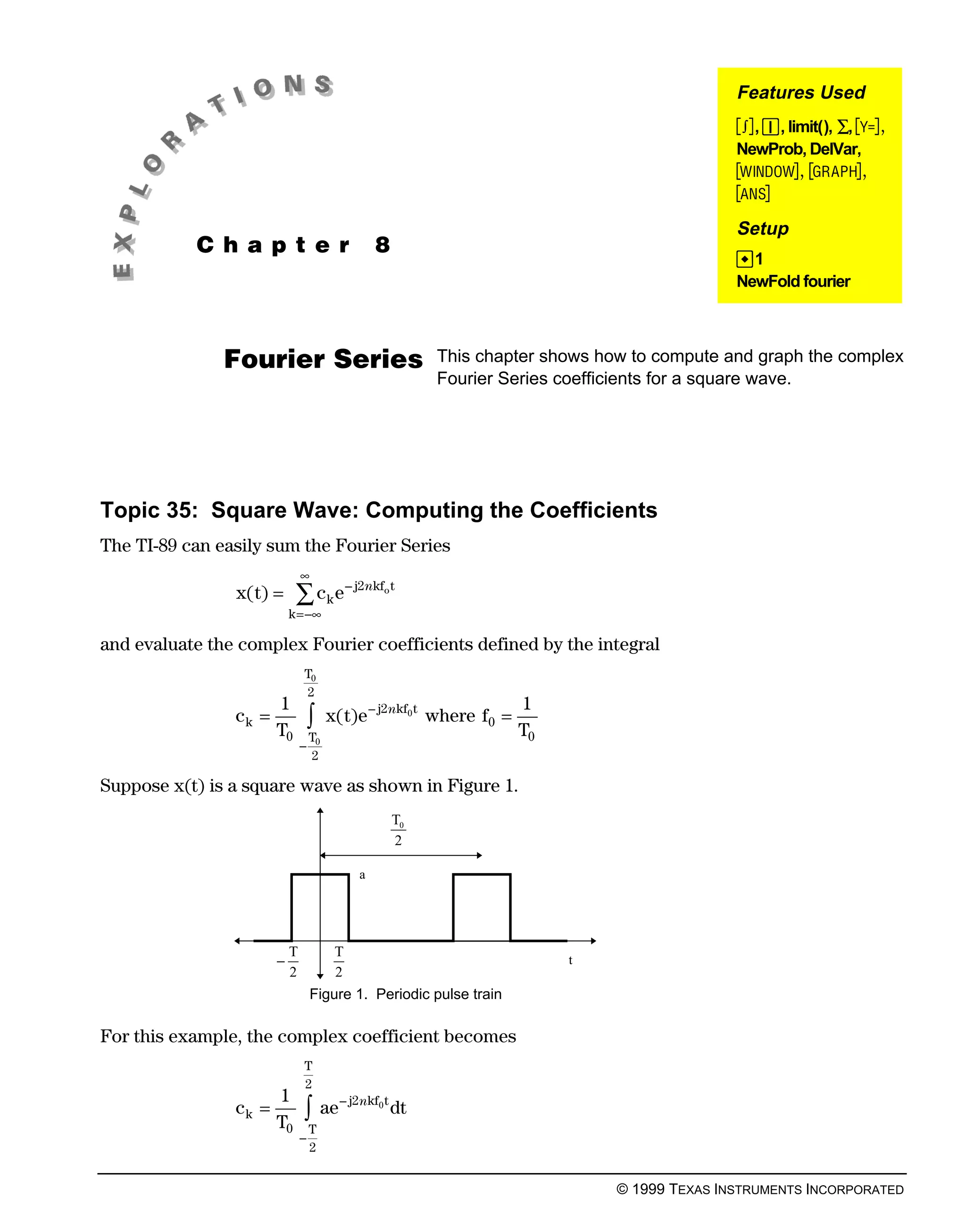
SlideShare a Scribd company logo
1 of 6
Download to read offline
Features Used
                                                                                                 <, Í, limit(), ∑, #,
                                                                                                 NewProb, DelVar,
                                                                                                 $, %,
                                                                                                 ±
                                                                                                 Setup
           C h a p t e r                           8
                                                                                                 ¥1
                                                                                                 NewFold fourier
.


               Fourier Series                                This chapter shows how to compute and graph the complex
                                                             Fourier Series coefficients for a square wave.


Topic 35: Square Wave: Computing the Coefficients
The TI-89 can easily sum the Fourier Series
                               ∞
                x( t) =     ∑ ck e − j2nkf t        o

                           k =−∞

and evaluate the complex Fourier coefficients defined by the integral
                               T0
                               2
                       1                                                 1
                ck =
                       T0
                               −
                                   z
                                   T0
                                         x( t)e − j2 nkf0 t where f0 =
                                                                         T0
                                   2

Suppose x(t) is a square wave as shown in Figure 1.
                                                        T0
                                                        2

                                               a


                           T              T
                       −                                                      t
                           2              2
                                   Figure 1. Periodic pulse train

For this example, the complex coefficient becomes
                               T
                               2
                       1
                ck =
                       T0
                               z
                               −
                                   T
                                        ae − j2 nkf0 t dt

                                   2


                                                                                  © 1999 TEXAS INSTRUMENTS INCORPORATED
78     ELECTRICAL ENGINEERING APPLICATIONS WITH THE TI-89


1.   Clear the TI-89 by pressing 2 ˆ 2:NewProb ¸.
2.   Three variable substitutions are needed before entering
     the expression for the complex coefficient. T0 is entered
     as t00 (t0 is reserved), T is entered as tt (t and T are the
     same on the TI-89), and j is ) which is entered as
     2 ). Before entering the equation, any previous
     values of the variables used must be deleted as shown
                                                                     (1)
     in screen 1.
     ½ DelVar t00 b tt b f0
3.   Enter the integral (screen 2).
     1 e t00 2 < a ¥ s · 2 ) 2 2 T k p f0 p t d
     b t b · tt e 2 b tt e 2 d § tmp


                                                                     (2)
                                                                     Note: If a Domain Error message
                                                                     appears, try switching to radian
                                                                     angle mode by pressing 3 and
                                                                     selecting RADIAN.
4.   Next plot the coefficients. To do this, pick values for a,
     f0 (which sets t00 also), and tt. Try the values shown in
     screen 3.


                                                                     (3)
5.   In this example, a is set to 1 and f0 to 1000 Hz. With tt set
     to t00/2, the duty cycle is ½ so the square wave will be
     “on” half the time. Display the value of tmp (top of
     screen 4).
6.   Now save the formula for the coefficient in a function
     called c(k) as shown in screen 4.                               (4)

     2±§cckd
     Using the answer from the integral ensures that the
     value stored in c(k) is the result of the integral, not the
     integral itself. If the integral is saved, it is reevaluated
     every time a coefficient is computed. With c(k) stored
     as a function, the integral is evaluated once and the
     resulting formula is used each time a coefficient value
     is needed.


© 1999 TEXAS INSTRUMENTS INCORPORATED
CHAPTER 8: FOURIER SERIES   79

7.   Check a few data points as shown in screen 5.


                                                                   (5)
8.   All the coefficients look fine except for k=0. The
     equation for c(k) shows that for k=0 the result is 0/0.
     The correct value can be found by using limit( )
     (screen 6).
     ½ limit( c c k d b k b 0 d
                                                                   (6)
     The correct value of c(k) for k=0 is ½. This makes sense
     since the square wave is turned on half the time with an
     average value of ½.
9.   Use the when( ) function to define c(k) so that the k=0
     case is calculated correctly (screen 7).
     ½ when( k Á 0 b 1 e 2 b c c k d d § cc c k
     d
     The value of c(k) valid for all k is stored in cc(k). Now
                                                                   (7)
     the coefficients can be plotted.
10. Set the Graph mode to SEQUENCE (3 B 4:SEQUENCE
    ¸), press ¥ #, and enter cc(n) as the sequence to
     be plotted, as shown in screen 8. Note that the sequence
     plot mode uses the variable n.

                                                                   (8)
11. Press ¥ $ to set the plot range as shown in                   Note: nmin must be greater than or
     screen 9.                                                    equal to 0.


                                                                   (9)
12. Press ¥ % to see the results as shown in screen 10.

     The graph also could be done in Function graphing
     mode. Sequence graphing mode is chosen to emphasize
     that the coefficients only appear at integer values.

                                                                  (10)


                                                                 © 1999 TEXAS INSTRUMENTS INCORPORATED
80     ELECTRICAL ENGINEERING APPLICATIONS WITH THE TI-89


Topic 36: Square Wave: Constructing the Wave from the Coefficients
The original signal can be rebuilt from the coefficients by using
                             ∞        − j2 πkf0 t
                  x( t) =    ∑ ck e
                            k =−∞

1.   To do this, return to the Home screen and enter the
     expression as shown in screen 11.
     ½ G( cc c k d ¥ s 2 ) 2 2 T k p f0 p t
     dbkb·3b3d
     Notice that the TI-89 applied Euler’s Identity to terms of
                                                                    (11)
     the form eiθ+ eNiθ to get 2cos(θ).
     The complete output is
                   −2 cos(6000πt ) 2 cos(2000πt )
                                  +               +1/ 2
                         3π              π
2.   Save the result as y1(x), screen 12.
     2 ± Í t Á x § y1 c x d                                         (12)

3.   Switch the Graph mode to FUNCTION by pressing 3
     B 1:FUNCTION ¸. Then press ¥ # to verify that
     the equation is entered in the Y= Editor (screen 13).


                                                                    (13)
4.   Press ¥ $ and set the plot range as shown in
     screen 14.


                                                                    (14)
5.   Press ¥ % to see the graph of x(t) as shown in
     screen 15.
     It’s not quite a square wave, but it’s not too bad for
     using only 5 non-zero coefficients. Recall that c(-3),
     c(-1), c(0), c(1) and c(3) are non-zero; c(-2)=c(2)=0.
                                                                    (15)
6.   To get a more accurate representation, include more
     coefficients of the series. On the Home screen, change
     the summation range to -5 to 5 as shown in screen 16.
     ½ G( cc c k d ¥ s 2 ) 2 2 T k p f0 p t
     dbkb·5b5d
                                                                    (16)


© 1999 TEXAS INSTRUMENTS INCORPORATED
CHAPTER 8: FOURIER SERIES   81

     The output for the 5-term series is
                  2 cos(10000πt ) 2 cos(6000πt )
                                  −
                        5π                  3π
                    2 cos(2000πt )
                  +                + 1 / 2.
                          π
                                                                   (17)
7.   Save the result in y2(x) as shown in screen 17.
     2 ± Í t Á x § y2 c x d
8.   Press ¥ %. Screen 18 compares the resulting graph
     of the sum for k=.5 to 5 with the original graph for the
     sum of k=.3 to 3. The new result more closely
     represents a square wave because the sum more closely
     represents a square wave as the number of terms
     increases. With an infinite number of terms, the sum
                                                                   (18)
     exactly represents the square wave.
Tips and Generalizations
The TI-89 can easily find the Fourier Series coefficients in closed form for many periodic signals.
In this chapter, c(k) could be expressed as a simple equation. More complex signals may not have a
closed form solution. In these cases, use numeric integration (nInt) to find each of the coefficients.
Chapter 9 adds a new dimension by showing how the TI-89 can manipulate vectors.


                                                                 © 1999 TEXAS INSTRUMENTS INCORPORATED
82    ELECTRICAL ENGINEERING APPLICATIONS WITH THE TI-89


© 1999 TEXAS INSTRUMENTS INCORPORATED

More Related Content

What's hot

Computer Capacity & Performance Evaluation Sheets
Computer Capacity & Performance Evaluation SheetsComputer Capacity & Performance Evaluation Sheets
Computer Capacity & Performance Evaluation SheetsDeru Sudibyo
 
Dsp U Lec07 Realization Of Discrete Time Systems
Dsp U   Lec07 Realization Of Discrete Time SystemsDsp U   Lec07 Realization Of Discrete Time Systems
Dsp U Lec07 Realization Of Discrete Time Systemstaha25
 
Case Study (All)
Case Study (All)Case Study (All)
Case Study (All)gudeyi
 
Isi and nyquist criterion
Isi and nyquist criterionIsi and nyquist criterion
Isi and nyquist criterionsrkrishna341
 
Correlative level coding
Correlative level codingCorrelative level coding
Correlative level codingsrkrishna341
 
Phase de-trending of modulated signals
Phase de-trending of modulated signalsPhase de-trending of modulated signals
Phase de-trending of modulated signalsNMDG NV
 
2010 APS_ Broadband Characteristics of A Dome Dipole Antenna
2010 APS_ Broadband Characteristics of A Dome Dipole Antenna2010 APS_ Broadband Characteristics of A Dome Dipole Antenna
2010 APS_ Broadband Characteristics of A Dome Dipole AntennaJing Zhao
 
IGARSS2011 FR3.T08.3 BenDavid.pdf
IGARSS2011 FR3.T08.3 BenDavid.pdfIGARSS2011 FR3.T08.3 BenDavid.pdf
IGARSS2011 FR3.T08.3 BenDavid.pdfgrssieee
 
Chapter 2 signals and spectra,
Chapter 2   signals and spectra,Chapter 2   signals and spectra,
Chapter 2 signals and spectra,nahrain university
 
DSP_FOEHU - MATLAB 02 - The Discrete-time Fourier Analysis
DSP_FOEHU - MATLAB 02 - The Discrete-time Fourier AnalysisDSP_FOEHU - MATLAB 02 - The Discrete-time Fourier Analysis
DSP_FOEHU - MATLAB 02 - The Discrete-time Fourier AnalysisAmr E. Mohamed
 

What's hot (20)

quantization
quantizationquantization
quantization
 
Antnrfld
AntnrfldAntnrfld
Antnrfld
 
Computer Capacity & Performance Evaluation Sheets
Computer Capacity & Performance Evaluation SheetsComputer Capacity & Performance Evaluation Sheets
Computer Capacity & Performance Evaluation Sheets
 
Dsp U Lec07 Realization Of Discrete Time Systems
Dsp U   Lec07 Realization Of Discrete Time SystemsDsp U   Lec07 Realization Of Discrete Time Systems
Dsp U Lec07 Realization Of Discrete Time Systems
 
Hw4sol
Hw4solHw4sol
Hw4sol
 
Matched filter
Matched filterMatched filter
Matched filter
 
Case Study (All)
Case Study (All)Case Study (All)
Case Study (All)
 
Isi and nyquist criterion
Isi and nyquist criterionIsi and nyquist criterion
Isi and nyquist criterion
 
Chapter6 sampling
Chapter6 samplingChapter6 sampling
Chapter6 sampling
 
Correlative level coding
Correlative level codingCorrelative level coding
Correlative level coding
 
Phase de-trending of modulated signals
Phase de-trending of modulated signalsPhase de-trending of modulated signals
Phase de-trending of modulated signals
 
2010 APS_ Broadband Characteristics of A Dome Dipole Antenna
2010 APS_ Broadband Characteristics of A Dome Dipole Antenna2010 APS_ Broadband Characteristics of A Dome Dipole Antenna
2010 APS_ Broadband Characteristics of A Dome Dipole Antenna
 
IGARSS2011 FR3.T08.3 BenDavid.pdf
IGARSS2011 FR3.T08.3 BenDavid.pdfIGARSS2011 FR3.T08.3 BenDavid.pdf
IGARSS2011 FR3.T08.3 BenDavid.pdf
 
Chapter 2 signals and spectra,
Chapter 2   signals and spectra,Chapter 2   signals and spectra,
Chapter 2 signals and spectra,
 
Properties of Fourier transform
Properties of Fourier transformProperties of Fourier transform
Properties of Fourier transform
 
Sampling
SamplingSampling
Sampling
 
DSP_FOEHU - MATLAB 02 - The Discrete-time Fourier Analysis
DSP_FOEHU - MATLAB 02 - The Discrete-time Fourier AnalysisDSP_FOEHU - MATLAB 02 - The Discrete-time Fourier Analysis
DSP_FOEHU - MATLAB 02 - The Discrete-time Fourier Analysis
 
Fourier transform
Fourier transformFourier transform
Fourier transform
 
F0543645
F0543645F0543645
F0543645
 
Solved problems
Solved problemsSolved problems
Solved problems
 

Similar to 08 fouri

Pid En Un Pic16 F684
Pid En Un Pic16 F684Pid En Un Pic16 F684
Pid En Un Pic16 F684quadrocopter
 
Pid En Un Pic16 F684
Pid En Un Pic16 F684Pid En Un Pic16 F684
Pid En Un Pic16 F684quadrocopter
 
The convenience yield implied by quadratic volatility smiles presentation [...
The convenience yield implied by quadratic volatility smiles   presentation [...The convenience yield implied by quadratic volatility smiles   presentation [...
The convenience yield implied by quadratic volatility smiles presentation [...yigalbt
 
ECNG 3015 Power System Protection
ECNG 3015    Power System ProtectionECNG 3015    Power System Protection
ECNG 3015 Power System ProtectionChandrabhan Sharma
 
Hull White model presentation
Hull White model presentationHull White model presentation
Hull White model presentationStephan Chang
 
LAB05ex1.mfunction LAB05ex1m = 1; .docx
LAB05ex1.mfunction LAB05ex1m = 1;                          .docxLAB05ex1.mfunction LAB05ex1m = 1;                          .docx
LAB05ex1.mfunction LAB05ex1m = 1; .docxsmile790243
 
MATLAB sessions Laboratory 6MAT 275 Laboratory 6Forced .docx
MATLAB sessions Laboratory 6MAT 275 Laboratory 6Forced .docxMATLAB sessions Laboratory 6MAT 275 Laboratory 6Forced .docx
MATLAB sessions Laboratory 6MAT 275 Laboratory 6Forced .docxandreecapon
 
Local Volatility 1
Local Volatility 1Local Volatility 1
Local Volatility 1Ilya Gikhman
 
Study of the variation of power loss with frequency along a rectangular
Study of the variation of power loss with frequency along a rectangularStudy of the variation of power loss with frequency along a rectangular
Study of the variation of power loss with frequency along a rectangularIAEME Publication
 
WaveletTutorial.pdf
WaveletTutorial.pdfWaveletTutorial.pdf
WaveletTutorial.pdfshreyassr9
 
Robust adaptive integral backstepping control and its implementation on
Robust adaptive integral backstepping control and its implementation onRobust adaptive integral backstepping control and its implementation on
Robust adaptive integral backstepping control and its implementation onShubhobrata Rudra
 
Supplement to local voatility
Supplement to local voatilitySupplement to local voatility
Supplement to local voatilityIlya Gikhman
 
SCRUTINY TO THE NON-AXIALLY DEFORMATIONS OF AN ELASTIC FOUNDATION ON A CYLIND...
SCRUTINY TO THE NON-AXIALLY DEFORMATIONS OF AN ELASTIC FOUNDATION ON A CYLIND...SCRUTINY TO THE NON-AXIALLY DEFORMATIONS OF AN ELASTIC FOUNDATION ON A CYLIND...
SCRUTINY TO THE NON-AXIALLY DEFORMATIONS OF AN ELASTIC FOUNDATION ON A CYLIND...P singh
 
Matlab 3
Matlab 3Matlab 3
Matlab 3asguna
 
Heat Map Modeling Using Resistive Network
Heat Map Modeling Using Resistive NetworkHeat Map Modeling Using Resistive Network
Heat Map Modeling Using Resistive Networkssurgnier
 

Similar to 08 fouri (20)

Pid En Un Pic16 F684
Pid En Un Pic16 F684Pid En Un Pic16 F684
Pid En Un Pic16 F684
 
Pid En Un Pic16 F684
Pid En Un Pic16 F684Pid En Un Pic16 F684
Pid En Un Pic16 F684
 
36
3636
36
 
1568973267 effect of multi-tone
1568973267 effect of multi-tone1568973267 effect of multi-tone
1568973267 effect of multi-tone
 
The convenience yield implied by quadratic volatility smiles presentation [...
The convenience yield implied by quadratic volatility smiles   presentation [...The convenience yield implied by quadratic volatility smiles   presentation [...
The convenience yield implied by quadratic volatility smiles presentation [...
 
ECNG 3015 Power System Protection
ECNG 3015    Power System ProtectionECNG 3015    Power System Protection
ECNG 3015 Power System Protection
 
Hull White model presentation
Hull White model presentationHull White model presentation
Hull White model presentation
 
ACS 22LIE12 lab Manul.docx
ACS 22LIE12 lab Manul.docxACS 22LIE12 lab Manul.docx
ACS 22LIE12 lab Manul.docx
 
LAB05ex1.mfunction LAB05ex1m = 1; .docx
LAB05ex1.mfunction LAB05ex1m = 1;                          .docxLAB05ex1.mfunction LAB05ex1m = 1;                          .docx
LAB05ex1.mfunction LAB05ex1m = 1; .docx
 
Lect 02
Lect 02Lect 02
Lect 02
 
MATLAB sessions Laboratory 6MAT 275 Laboratory 6Forced .docx
MATLAB sessions Laboratory 6MAT 275 Laboratory 6Forced .docxMATLAB sessions Laboratory 6MAT 275 Laboratory 6Forced .docx
MATLAB sessions Laboratory 6MAT 275 Laboratory 6Forced .docx
 
Local Volatility 1
Local Volatility 1Local Volatility 1
Local Volatility 1
 
Study of the variation of power loss with frequency along a rectangular
Study of the variation of power loss with frequency along a rectangularStudy of the variation of power loss with frequency along a rectangular
Study of the variation of power loss with frequency along a rectangular
 
WaveletTutorial.pdf
WaveletTutorial.pdfWaveletTutorial.pdf
WaveletTutorial.pdf
 
job scheduling
job schedulingjob scheduling
job scheduling
 
Robust adaptive integral backstepping control and its implementation on
Robust adaptive integral backstepping control and its implementation onRobust adaptive integral backstepping control and its implementation on
Robust adaptive integral backstepping control and its implementation on
 
Supplement to local voatility
Supplement to local voatilitySupplement to local voatility
Supplement to local voatility
 
SCRUTINY TO THE NON-AXIALLY DEFORMATIONS OF AN ELASTIC FOUNDATION ON A CYLIND...
SCRUTINY TO THE NON-AXIALLY DEFORMATIONS OF AN ELASTIC FOUNDATION ON A CYLIND...SCRUTINY TO THE NON-AXIALLY DEFORMATIONS OF AN ELASTIC FOUNDATION ON A CYLIND...
SCRUTINY TO THE NON-AXIALLY DEFORMATIONS OF AN ELASTIC FOUNDATION ON A CYLIND...
 
Matlab 3
Matlab 3Matlab 3
Matlab 3
 
Heat Map Modeling Using Resistive Network
Heat Map Modeling Using Resistive NetworkHeat Map Modeling Using Resistive Network
Heat Map Modeling Using Resistive Network
 

Recently uploaded

Powerpoint exploring the locations used in television show Time Clash
Powerpoint exploring the locations used in television show Time ClashPowerpoint exploring the locations used in television show Time Clash
Powerpoint exploring the locations used in television show Time Clashcharlottematthew16
 
My Hashitalk Indonesia April 2024 Presentation
My Hashitalk Indonesia April 2024 PresentationMy Hashitalk Indonesia April 2024 Presentation
My Hashitalk Indonesia April 2024 PresentationRidwan Fadjar
 
Developer Data Modeling Mistakes: From Postgres to NoSQL
Developer Data Modeling Mistakes: From Postgres to NoSQLDeveloper Data Modeling Mistakes: From Postgres to NoSQL
Developer Data Modeling Mistakes: From Postgres to NoSQLScyllaDB
 
SAP Build Work Zone - Overview L2-L3.pptx
SAP Build Work Zone - Overview L2-L3.pptxSAP Build Work Zone - Overview L2-L3.pptx
SAP Build Work Zone - Overview L2-L3.pptxNavinnSomaal
 
Streamlining Python Development: A Guide to a Modern Project Setup
Streamlining Python Development: A Guide to a Modern Project SetupStreamlining Python Development: A Guide to a Modern Project Setup
Streamlining Python Development: A Guide to a Modern Project SetupFlorian Wilhelm
 
SQL Database Design For Developers at php[tek] 2024
SQL Database Design For Developers at php[tek] 2024SQL Database Design For Developers at php[tek] 2024
SQL Database Design For Developers at php[tek] 2024Scott Keck-Warren
 
Ensuring Technical Readiness For Copilot in Microsoft 365
Ensuring Technical Readiness For Copilot in Microsoft 365Ensuring Technical Readiness For Copilot in Microsoft 365
Ensuring Technical Readiness For Copilot in Microsoft 3652toLead Limited
 
Transcript: New from BookNet Canada for 2024: BNC CataList - Tech Forum 2024
Transcript: New from BookNet Canada for 2024: BNC CataList - Tech Forum 2024Transcript: New from BookNet Canada for 2024: BNC CataList - Tech Forum 2024
Transcript: New from BookNet Canada for 2024: BNC CataList - Tech Forum 2024BookNet Canada
 
Designing IA for AI - Information Architecture Conference 2024
Designing IA for AI - Information Architecture Conference 2024Designing IA for AI - Information Architecture Conference 2024
Designing IA for AI - Information Architecture Conference 2024Enterprise Knowledge
 
"Federated learning: out of reach no matter how close",Oleksandr Lapshyn
"Federated learning: out of reach no matter how close",Oleksandr Lapshyn"Federated learning: out of reach no matter how close",Oleksandr Lapshyn
"Federated learning: out of reach no matter how close",Oleksandr LapshynFwdays
 
My INSURER PTE LTD - Insurtech Innovation Award 2024
My INSURER PTE LTD - Insurtech Innovation Award 2024My INSURER PTE LTD - Insurtech Innovation Award 2024
My INSURER PTE LTD - Insurtech Innovation Award 2024The Digital Insurer
 
CloudStudio User manual (basic edition):
CloudStudio User manual (basic edition):CloudStudio User manual (basic edition):
CloudStudio User manual (basic edition):comworks
 
Scanning the Internet for External Cloud Exposures via SSL Certs
Scanning the Internet for External Cloud Exposures via SSL CertsScanning the Internet for External Cloud Exposures via SSL Certs
Scanning the Internet for External Cloud Exposures via SSL CertsRizwan Syed
 
Tech-Forward - Achieving Business Readiness For Copilot in Microsoft 365
Tech-Forward - Achieving Business Readiness For Copilot in Microsoft 365Tech-Forward - Achieving Business Readiness For Copilot in Microsoft 365
Tech-Forward - Achieving Business Readiness For Copilot in Microsoft 3652toLead Limited
 
Beyond Boundaries: Leveraging No-Code Solutions for Industry Innovation
Beyond Boundaries: Leveraging No-Code Solutions for Industry InnovationBeyond Boundaries: Leveraging No-Code Solutions for Industry Innovation
Beyond Boundaries: Leveraging No-Code Solutions for Industry InnovationSafe Software
 
Artificial intelligence in cctv survelliance.pptx
Artificial intelligence in cctv survelliance.pptxArtificial intelligence in cctv survelliance.pptx
Artificial intelligence in cctv survelliance.pptxhariprasad279825
 
Human Factors of XR: Using Human Factors to Design XR Systems
Human Factors of XR: Using Human Factors to Design XR SystemsHuman Factors of XR: Using Human Factors to Design XR Systems
Human Factors of XR: Using Human Factors to Design XR SystemsMark Billinghurst
 
Commit 2024 - Secret Management made easy
Commit 2024 - Secret Management made easyCommit 2024 - Secret Management made easy
Commit 2024 - Secret Management made easyAlfredo García Lavilla
 
Understanding the Laravel MVC Architecture
Understanding the Laravel MVC ArchitectureUnderstanding the Laravel MVC Architecture
Understanding the Laravel MVC ArchitecturePixlogix Infotech
 
"Debugging python applications inside k8s environment", Andrii Soldatenko
"Debugging python applications inside k8s environment", Andrii Soldatenko"Debugging python applications inside k8s environment", Andrii Soldatenko
"Debugging python applications inside k8s environment", Andrii SoldatenkoFwdays
 

Recently uploaded (20)

Powerpoint exploring the locations used in television show Time Clash
Powerpoint exploring the locations used in television show Time ClashPowerpoint exploring the locations used in television show Time Clash
Powerpoint exploring the locations used in television show Time Clash
 
My Hashitalk Indonesia April 2024 Presentation
My Hashitalk Indonesia April 2024 PresentationMy Hashitalk Indonesia April 2024 Presentation
My Hashitalk Indonesia April 2024 Presentation
 
Developer Data Modeling Mistakes: From Postgres to NoSQL
Developer Data Modeling Mistakes: From Postgres to NoSQLDeveloper Data Modeling Mistakes: From Postgres to NoSQL
Developer Data Modeling Mistakes: From Postgres to NoSQL
 
SAP Build Work Zone - Overview L2-L3.pptx
SAP Build Work Zone - Overview L2-L3.pptxSAP Build Work Zone - Overview L2-L3.pptx
SAP Build Work Zone - Overview L2-L3.pptx
 
Streamlining Python Development: A Guide to a Modern Project Setup
Streamlining Python Development: A Guide to a Modern Project SetupStreamlining Python Development: A Guide to a Modern Project Setup
Streamlining Python Development: A Guide to a Modern Project Setup
 
SQL Database Design For Developers at php[tek] 2024
SQL Database Design For Developers at php[tek] 2024SQL Database Design For Developers at php[tek] 2024
SQL Database Design For Developers at php[tek] 2024
 
Ensuring Technical Readiness For Copilot in Microsoft 365
Ensuring Technical Readiness For Copilot in Microsoft 365Ensuring Technical Readiness For Copilot in Microsoft 365
Ensuring Technical Readiness For Copilot in Microsoft 365
 
Transcript: New from BookNet Canada for 2024: BNC CataList - Tech Forum 2024
Transcript: New from BookNet Canada for 2024: BNC CataList - Tech Forum 2024Transcript: New from BookNet Canada for 2024: BNC CataList - Tech Forum 2024
Transcript: New from BookNet Canada for 2024: BNC CataList - Tech Forum 2024
 
Designing IA for AI - Information Architecture Conference 2024
Designing IA for AI - Information Architecture Conference 2024Designing IA for AI - Information Architecture Conference 2024
Designing IA for AI - Information Architecture Conference 2024
 
"Federated learning: out of reach no matter how close",Oleksandr Lapshyn
"Federated learning: out of reach no matter how close",Oleksandr Lapshyn"Federated learning: out of reach no matter how close",Oleksandr Lapshyn
"Federated learning: out of reach no matter how close",Oleksandr Lapshyn
 
My INSURER PTE LTD - Insurtech Innovation Award 2024
My INSURER PTE LTD - Insurtech Innovation Award 2024My INSURER PTE LTD - Insurtech Innovation Award 2024
My INSURER PTE LTD - Insurtech Innovation Award 2024
 
CloudStudio User manual (basic edition):
CloudStudio User manual (basic edition):CloudStudio User manual (basic edition):
CloudStudio User manual (basic edition):
 
Scanning the Internet for External Cloud Exposures via SSL Certs
Scanning the Internet for External Cloud Exposures via SSL CertsScanning the Internet for External Cloud Exposures via SSL Certs
Scanning the Internet for External Cloud Exposures via SSL Certs
 
Tech-Forward - Achieving Business Readiness For Copilot in Microsoft 365
Tech-Forward - Achieving Business Readiness For Copilot in Microsoft 365Tech-Forward - Achieving Business Readiness For Copilot in Microsoft 365
Tech-Forward - Achieving Business Readiness For Copilot in Microsoft 365
 
Beyond Boundaries: Leveraging No-Code Solutions for Industry Innovation
Beyond Boundaries: Leveraging No-Code Solutions for Industry InnovationBeyond Boundaries: Leveraging No-Code Solutions for Industry Innovation
Beyond Boundaries: Leveraging No-Code Solutions for Industry Innovation
 
Artificial intelligence in cctv survelliance.pptx
Artificial intelligence in cctv survelliance.pptxArtificial intelligence in cctv survelliance.pptx
Artificial intelligence in cctv survelliance.pptx
 
Human Factors of XR: Using Human Factors to Design XR Systems
Human Factors of XR: Using Human Factors to Design XR SystemsHuman Factors of XR: Using Human Factors to Design XR Systems
Human Factors of XR: Using Human Factors to Design XR Systems
 
Commit 2024 - Secret Management made easy
Commit 2024 - Secret Management made easyCommit 2024 - Secret Management made easy
Commit 2024 - Secret Management made easy
 
Understanding the Laravel MVC Architecture
Understanding the Laravel MVC ArchitectureUnderstanding the Laravel MVC Architecture
Understanding the Laravel MVC Architecture
 
"Debugging python applications inside k8s environment", Andrii Soldatenko
"Debugging python applications inside k8s environment", Andrii Soldatenko"Debugging python applications inside k8s environment", Andrii Soldatenko
"Debugging python applications inside k8s environment", Andrii Soldatenko
 

08 fouri

  • 1. Features Used <, Í, limit(), ∑, #, NewProb, DelVar, $, %, ± Setup C h a p t e r 8 ¥1 NewFold fourier . Fourier Series This chapter shows how to compute and graph the complex Fourier Series coefficients for a square wave. Topic 35: Square Wave: Computing the Coefficients The TI-89 can easily sum the Fourier Series ∞ x( t) = ∑ ck e − j2nkf t o k =−∞ and evaluate the complex Fourier coefficients defined by the integral T0 2 1 1 ck = T0 − z T0 x( t)e − j2 nkf0 t where f0 = T0 2 Suppose x(t) is a square wave as shown in Figure 1. T0 2 a T T − t 2 2 Figure 1. Periodic pulse train For this example, the complex coefficient becomes T 2 1 ck = T0 z − T ae − j2 nkf0 t dt 2 © 1999 TEXAS INSTRUMENTS INCORPORATED
  • 2. 78 ELECTRICAL ENGINEERING APPLICATIONS WITH THE TI-89 1. Clear the TI-89 by pressing 2 ˆ 2:NewProb ¸. 2. Three variable substitutions are needed before entering the expression for the complex coefficient. T0 is entered as t00 (t0 is reserved), T is entered as tt (t and T are the same on the TI-89), and j is ) which is entered as 2 ). Before entering the equation, any previous values of the variables used must be deleted as shown (1) in screen 1. ½ DelVar t00 b tt b f0 3. Enter the integral (screen 2). 1 e t00 2 < a ¥ s · 2 ) 2 2 T k p f0 p t d b t b · tt e 2 b tt e 2 d § tmp (2) Note: If a Domain Error message appears, try switching to radian angle mode by pressing 3 and selecting RADIAN. 4. Next plot the coefficients. To do this, pick values for a, f0 (which sets t00 also), and tt. Try the values shown in screen 3. (3) 5. In this example, a is set to 1 and f0 to 1000 Hz. With tt set to t00/2, the duty cycle is ½ so the square wave will be “on” half the time. Display the value of tmp (top of screen 4). 6. Now save the formula for the coefficient in a function called c(k) as shown in screen 4. (4) 2±§cckd Using the answer from the integral ensures that the value stored in c(k) is the result of the integral, not the integral itself. If the integral is saved, it is reevaluated every time a coefficient is computed. With c(k) stored as a function, the integral is evaluated once and the resulting formula is used each time a coefficient value is needed. © 1999 TEXAS INSTRUMENTS INCORPORATED
  • 3. CHAPTER 8: FOURIER SERIES 79 7. Check a few data points as shown in screen 5. (5) 8. All the coefficients look fine except for k=0. The equation for c(k) shows that for k=0 the result is 0/0. The correct value can be found by using limit( ) (screen 6). ½ limit( c c k d b k b 0 d (6) The correct value of c(k) for k=0 is ½. This makes sense since the square wave is turned on half the time with an average value of ½. 9. Use the when( ) function to define c(k) so that the k=0 case is calculated correctly (screen 7). ½ when( k Á 0 b 1 e 2 b c c k d d § cc c k d The value of c(k) valid for all k is stored in cc(k). Now (7) the coefficients can be plotted. 10. Set the Graph mode to SEQUENCE (3 B 4:SEQUENCE ¸), press ¥ #, and enter cc(n) as the sequence to be plotted, as shown in screen 8. Note that the sequence plot mode uses the variable n. (8) 11. Press ¥ $ to set the plot range as shown in Note: nmin must be greater than or screen 9. equal to 0. (9) 12. Press ¥ % to see the results as shown in screen 10. The graph also could be done in Function graphing mode. Sequence graphing mode is chosen to emphasize that the coefficients only appear at integer values. (10) © 1999 TEXAS INSTRUMENTS INCORPORATED
  • 4. 80 ELECTRICAL ENGINEERING APPLICATIONS WITH THE TI-89 Topic 36: Square Wave: Constructing the Wave from the Coefficients The original signal can be rebuilt from the coefficients by using ∞ − j2 πkf0 t x( t) = ∑ ck e k =−∞ 1. To do this, return to the Home screen and enter the expression as shown in screen 11. ½ G( cc c k d ¥ s 2 ) 2 2 T k p f0 p t dbkb·3b3d Notice that the TI-89 applied Euler’s Identity to terms of (11) the form eiθ+ eNiθ to get 2cos(θ). The complete output is −2 cos(6000πt ) 2 cos(2000πt ) + +1/ 2 3π π 2. Save the result as y1(x), screen 12. 2 ± Í t Á x § y1 c x d (12) 3. Switch the Graph mode to FUNCTION by pressing 3 B 1:FUNCTION ¸. Then press ¥ # to verify that the equation is entered in the Y= Editor (screen 13). (13) 4. Press ¥ $ and set the plot range as shown in screen 14. (14) 5. Press ¥ % to see the graph of x(t) as shown in screen 15. It’s not quite a square wave, but it’s not too bad for using only 5 non-zero coefficients. Recall that c(-3), c(-1), c(0), c(1) and c(3) are non-zero; c(-2)=c(2)=0. (15) 6. To get a more accurate representation, include more coefficients of the series. On the Home screen, change the summation range to -5 to 5 as shown in screen 16. ½ G( cc c k d ¥ s 2 ) 2 2 T k p f0 p t dbkb·5b5d (16) © 1999 TEXAS INSTRUMENTS INCORPORATED
  • 5. CHAPTER 8: FOURIER SERIES 81 The output for the 5-term series is 2 cos(10000πt ) 2 cos(6000πt ) − 5π 3π 2 cos(2000πt ) + + 1 / 2. π (17) 7. Save the result in y2(x) as shown in screen 17. 2 ± Í t Á x § y2 c x d 8. Press ¥ %. Screen 18 compares the resulting graph of the sum for k=.5 to 5 with the original graph for the sum of k=.3 to 3. The new result more closely represents a square wave because the sum more closely represents a square wave as the number of terms increases. With an infinite number of terms, the sum (18) exactly represents the square wave. Tips and Generalizations The TI-89 can easily find the Fourier Series coefficients in closed form for many periodic signals. In this chapter, c(k) could be expressed as a simple equation. More complex signals may not have a closed form solution. In these cases, use numeric integration (nInt) to find each of the coefficients. Chapter 9 adds a new dimension by showing how the TI-89 can manipulate vectors. © 1999 TEXAS INSTRUMENTS INCORPORATED
  • 6. 82 ELECTRICAL ENGINEERING APPLICATIONS WITH THE TI-89 © 1999 TEXAS INSTRUMENTS INCORPORATED