I am Nicholas L. I am a Maths Assignment Expert at mathsassignmenthelp.com. I hold a Master's in Mathematics from the University of California. I have been helping students with their assignments for the past 10 years. I solve assignments related to Maths. Visit mathsassignmenthelp.com or email info@mathsassignmenthelp.com. You can also call +1 678 648 4277 for any assistance with Maths Assignments.

1. For any Assignment related queries, Call us at : - +1 678 648 4277
You can mail us at : - info@mathsassignmenthelp.com or
reach us at : - https://www.mathsassignmenthelp.com/

2. Problem 1:
Here are a few questions that you should be able to answer based only on 18.06:
a) Suppose that B is a Hermitian positive-definite matrix. Show that there is a unique
matrix √ B which is Hermitian positive-definite and has the property √( B)2 = B.
(Hint: use the diagonalization of B.)
(b) Suppose that A and B are Hermitian matrices and that B is positive-definite.
(i) Show that B−1A is similar (in the 18.06 sense) to a Hermitian matrix. (Hint: use your
answer from above.)
(ii) What does this tell you about the eigenvalues λ of B−1A , i.e. the solutions of B−1Ax =
λx?
(iii) Are the eigenvectors x orthogonal?
(iv) In Julia, make a random 5 × 5 real-symmetric matrix via A=rand(5,5); A = A+A’ and
a random 5 × 5 positive-definite matrix via B = rand(5,5); B = B’*B ... then check that
the eigenvalues of B−1A match your expectations from above via lambda,X =
eigvals(BA) (this will give an array lambda of the eigenvalues and a matrix X whose
columns are the eigenvectors).
mathsassignmenthelp.com

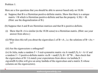
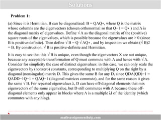
3. (v) Using your Julia result, what happens if you compute C = XT BX via C=X’*B*X?
You should notice that the matrix C is very special in some way. Show that the elements
Cij of C are a kind of “dot product” of the eigenvectors i and j, but with a factor of B in
the middle of the dot product.
(c) The solutions y(t) of the ODE y “− 2y ‘− cy = 0 are of the form y(t) =
for some constants C1 and C2 determined by
the initial conditions. Suppose that A is a real-symmetric 4×4 matrix with eigenvalues 3,
8, 15, 24 and corresponding eigenvectors x1, x2, . . . , x4, respectively.
(i) If x(t) solves the system of ODEs Ax with initial conditions x(0)
= a0 and x′ (0) = b0, write down the solution x(t) as a closed-form expression (no
matrix inverses or exponentials) in terms of the eigenvectors x1, x2, . . . , x4 and
a0 and b0. [Hint: expand x(t) in the basis of the eigenvectors with unknown
coefficients c1(t), . . . , c4(t), then plug into the ODE and solve for each coefficient
using the fact that the eigenvectors are _________.]
(ii) After a long time t ≫ 0, what do you expect the approximate form of the
solution to be?
mathsassignmenthelp.com

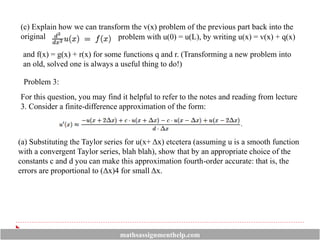
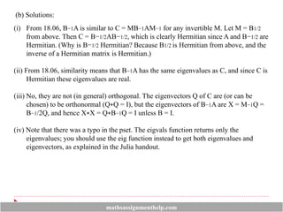
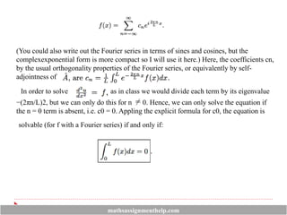
4. Problem 2:
In class, we considered the 1d Poisson equation
for the vector space of functions u(x) on x ∈ [0, L] with the “Dirichlet” boundary
conditions u(0) = u(L) = 0, and solved it in terms of the eigenfunctions of
(giving a Fourier sine series). Here, we will consider a couple of small variations on
this:
a) Suppose that we we change the boundary conditions to the periodic boundary
condition u(0) = u(L).
(i) What are the eigenfunctions of now?
(ii) Will Poisson’s equation have unique solutions? Why or why not?
(iii) Under what conditions (if any) on f(x) would a solution exist? (You can restrict
yourself to f with a convergent Fourier series.)
(b) If we instead consider
conditions v(0) = dx2 v(x) v(L) + 1, do these functions form a vector space? Why
or why not?
for functions v(x) with the boundary
mathsassignmenthelp.com

5. (c) Explain how we can transform the v(x) problem of the previous part back into the
original problem with u(0) = u(L), by writing u(x) = v(x) + q(x)
and f(x) = g(x) + r(x) for some functions q and r. (Transforming a new problem into
an old, solved one is always a useful thing to do!)
Problem 3:
For this question, you may find it helpful to refer to the notes and reading from lecture
3. Consider a finite-difference approximation of the form:
(a) Substituting the Taylor series for u(x+ Δx) etcetera (assuming u is a smooth function
with a convergent Taylor series, blah blah), show that by an appropriate choice of the
constants c and d you can make this approximation fourth-order accurate: that is, the
errors are proportional to (Δx)4 for small Δx.
mathsassignmenthelp.com

6. (b) Check your answer to the previous part by numerically computing u ′ (1) for u(x) =
sin(x), as a function of Δx, exactly as in the handout from class (refer to the notebook
posted in lecture 3 for the relevant Julia commands, and adapt them as needed). Verify
from your log-log plot of the |errors| versus Δx that you obtained the expected fourth-
order accuracy.
mathsassignmenthelp.com

7. Problem 1:
(a) Since it is Hermitian, B can be diagonalized: B = QΛQ∗, where Q is the matrix
whose columns are the eigenvectors (chosen orthonormal so that Q−1 = Q∗ ) and Λ is
the diagonal matrix of eigenvalues. Define √ Λ as the diagonal matrix of the (positive)
square roots of the eigenvalues, which is possible because the eigenvalues are > 0 (since
B is positive-definite). Then define √ B = Q √ ΛQ∗ , and by inspection we obtain (√ B)2
= B. By construction, √ B is positive-definite and Hermitian.
It is easy to see that this √ B is unique, even though the eigenvectors X are not unique,
because any acceptable transformation of Q must commute with Λ and hence with √ Λ.
Consider for simplicity the case of distinct eigenvalues: in this case, we can only scale the
eigenvectors by (nonzero) constants, corresponding to multiplying Q on the right by a
diagonal (nonsingular) matrix D. This gives the same B for any D, since QDΛ(QD)−1 =
QΛDD−1Q−1 = QΛQ−1 (diagonal matrices commute), and for the same reason it gives
the same √ B. For repeated eigenvalues λ, D can have off-diagonal elements that mix
eigenvectors of the same eigenvalue, but D still commutes with Λ because these off-
diagonal elements only appear in blocks where Λ is a multiple λI of the identity (which
commutes with anything).
mathsassignmenthelp.com

8. (b) Solutions:
(i) From 18.06, B−1A is similar to C = MB−1AM−1 for any invertible M. Let M = B1/2
from above. Then C = B−1/2AB−1/2, which is clearly Hermitian since A and B−1/2 are
Hermitian. (Why is B−1/2 Hermitian? Because B1/2 is Hermitian from above, and the
inverse of a Hermitian matrix is Hermitian.)
(ii) From 18.06, similarity means that B−1A has the same eigenvalues as C, and since C is
Hermitian these eigenvalues are real.
(iii) No, they are not (in general) orthogonal. The eigenvectors Q of C are (or can be
chosen) to be orthonormal (Q∗Q = I), but the eigenvectors of B−1A are X = M−1Q =
B−1/2Q, and hence X∗X = Q∗B−1Q = I unless B = I.
(iv) Note that there was a typo in the pset. The eigvals function returns only the
eigenvalues; you should use the eig function instead to get both eigenvalues and
eigenvectors, as explained in the Julia handout.
mathsassignmenthelp.com

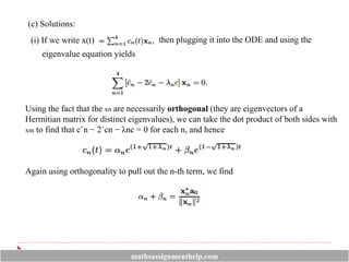
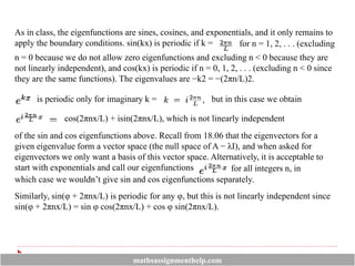
9. The array lambda that you obtain in Julia should be purely real, as expected. (You might
notice that the eigenvalues are in somewhat random order, e.g. I got -8.11,3.73,1.65,
1.502,0.443. This is a side effect of how eigenvalues of non-symmetric matrices are
computed in standard linear-algebra libraries like LAPACK.) You can check
orthogonality by computing X∗X via X’*X, and the result is not a diagonal matrix (or
even close to one), hence the vectors are not orthogonal.
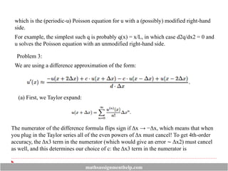
(v) When you compute C = X∗BX via C=X’*B*X, you should find that C is nearly
diagonal: the off-diagonal entries are all very close to zero (around 10−15 or less). They
would be exactly zero except for roundoff errors (as mentioned in class, computers keep
only around 15 significant digits). From the definition of matrix multiplication, the entry
Cij is given by the i-th row of X∗ multiplied by B, multiplied by the j-th column of X. ∗
But the j-th column X is the j-th eigenvector xj , and the i-th row of X∗ is x . Hence i ∗
Cij = xi Bxj, which looks like a dot product but with B in the middle. The fact that C
is diagonal means that which is a kind of orthogonality relation.
In fact, if we define the inner product (x, y) = x∗By, this is a perfectly good inner product
(it satisifies all the inner-product criteria because B is positive-definite), and we will see
in the next pset that B−1A is actually self-adjoint under this inner product. Hence it is no
surprise that we get real eigenvalues and orthogonal eigenvectors with respect to this
inner product.]
mathsassignmenthelp.com

10. (c) Solutions:
(i) If we write x(t) then plugging it into the ODE and using the
eigenvalue equation yields
Using the fact that the xn are necessarily orthogonal (they are eigenvectors of a
Hermitian matrix for distinct eigenvalues), we can take the dot product of both sides with
xm to find that c¨n − 2˙cn − λnc = 0 for each n, and hence
Again using orthogonality to pull out the n-th term, we find
mathsassignmenthelp.com

11. (note that we were not given that xn were normalized to unit length, and this is not
automatic) and hence we can solve for αn and βn to obtain:
(ii) After a long time, this expression will be dominated by the fastest growing term,
which √ (1+ 1+λn)t is the e term for λ4 = 24, hence:
Problem 2:
(a) Suppose that we we change the boundary conditions to the periodic boundary
condition u(0) = u(L).
mathsassignmenthelp.com

12. As in class, the eigenfunctions are sines, cosines, and exponentials, and it only remains to
apply the boundary conditions. sin(kx) is periodic if k = for n = 1, 2, . . . (excluding
n = 0 because we do not allow zero eigenfunctions and excluding n < 0 because they are
not linearly independent), and cos(kx) is periodic if n = 0, 1, 2, . . . (excluding n < 0 since
they are the same functions). The eigenvalues are −k2 = −(2πn/L)2.
is periodic only for imaginary k = but in this case we obtain
of the sin and cos eigenfunctions above. Recall from 18.06 that the eigenvectors for a
given eigenvalue form a vector space (the null space of A − λI), and when asked for
eigenvectors we only want a basis of this vector space. Alternatively, it is acceptable to
start with exponentials and call our eigenfunctions
cos(2πnx/L) + isin(2πnx/L), which is not linearly independent
which case we wouldn’t give sin and cos eigenfunctions separately.
for all integers n, in
Similarly, sin(φ + 2πnx/L) is periodic for any φ, but this is not linearly independent since
sin(φ + 2πnx/L) = sin φ cos(2πnx/L) + cos φ sin(2πnx/L).
mathsassignmenthelp.com

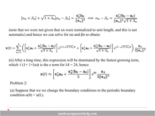
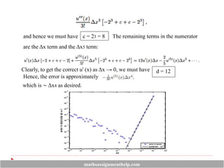
13. [Several of you were tempted to also allow sin(mπx/L) for odd m (not just the even m
considered above). At first glance, this seems like it satisfies the PDE and also has u(0) =
u(L) (= 0). Consider, for example, m = 1, i.e. sin(πx/L) solutions. This can’t be right,
however; e.g. it is not orthogonal to 1 = cos(0x), as required for self-adjoint problems.
The basic problem here is that if you consider the periodic extension of sin(πx/L), then it
doesn’t actually satisfy the PDE, because it has a slope discontinuity at the endpoints.
Another way of thinking about it is that periodic boundary conditions arise because we
have a PDE defined on a torus, e.g. diffusion around a circular tube, and in this case the
choice of endpoints is not unique—we can easily redefine our endpoints so that x = 0 is in
the “middle” of the domain, making it clearer that we can’t have a kink there. (This is one
of those cases where to be completely rigorous we would need to be a bit more careful
about defining the domain of our operator.)]
(ii) No, any solution will not be unique, because we now have a nonzero nullspace
spanned by the constant function u(x) = 1 (which is periodic):
Equivalently, we have a 0 eigenvalue corresponding to cos(2πnx/L) for n = 0 above.
(iii) As suggested, let us restrict ourselves to f(x) with a convergent Fourier series. That
is, as in class, we are expanding f(x) in terms of the eigenfunctions:
mathsassignmenthelp.com

14. (You could also write out the Fourier series in terms of sines and cosines, but the
complexexponential form is more compact so I will use it here.) Here, the coefficients cn,
by the usual orthogonality properties of the Fourier series, or equivalently by self-
adjointness of
In order to solve as in class we would divide each term by its eigenvalue
−(2πn/L)2, but we can only do this for n 0. Hence, we can only solve the equation if
the n = 0 term is absent, i.e. c0 = 0. Appling the explicit formula for c0, the equation is
solvable (for f with a Fourier series) if and only if:
mathsassignmenthelp.com

15. There are other ways to come to the same conclusion. For example, we could expand
u(x) in a Fourier series (i.e. in the eigenfunction basis), apply d2/dx2, and ask what is
the column space of d2/dx2? Again, we would find that upon taking the second
derivative the n = 0 (constant) term vanishes, and so the column space consist of Fourier
series missing a constant term.
The same reasoning works if you write out the Fourier series in terms of sin and cos
sums separately, in which case you find that f must be missing the n = 0 cosine term,
giving the same result.
(b) No. For example, the function 0 (which must be in any vector space) does not
satisy those boundary conditions. (Also adding functions doesn’t work, scaling them
by constants, etcetera.)
(c) We merely pick any twice-differentiable function q(x) with q(L) − q(0) = −1, in
which case u(L) − u(0) = [v(L) − v(0)] + [q(L) − q(0)] = 1 − 1 = 0 and u is periodic.
Then, plugging v = u − q into we obtain
mathsassignmenthelp.com

16. which is the (periodic-u) Poisson equation for u with a (possibly) modified right-hand
side.
For example, the simplest such q is probably q(x) = x/L, in which case d2q/dx2 = 0 and
u solves the Poisson equation with an unmodified right-hand side.
Problem 3:
We are using a difference approximation of the form:
(a) First, we Taylor expand:
The numerator of the difference formula flips sign if Δx → −Δx, which means that when
you plug in the Taylor series all of the even powers of Δx must cancel! To get 4th-order
accuracy, the Δx3 term in the numerator (which would give an error ∼ Δx2) must cancel
as well, and this determines our choice of c: the Δx3 term in the numerator is
mathsassignmenthelp.com

17. and hence we must have c = 23 = 8
are the Δx term and the Δx5 term:
The remaining terms in the numerator
Clearly, to get the correct u' (x) as Δx → 0, we must have d = 12
Hence, the error is approximately
which is ∼ Δx4 as desired.
mathsassignmenthelp.com

18. Figure 1: Actual vs. predicted error for problem 1(b), using fourth-order difference
approximation for u' (x) with u(x) = sin(x), at x = 1.
b) The Julia code is the same as in the handout, except now we compute our difference
approximation by the command: d = (-sin(x+2*dx) + 8*sin(x+dx) - 8*sin(x+dx) +
sin(x-2*dx)) ./ (12 * dx); the result is plotted in Fig. 1. Note that the error falls as a
straight line (a power law), until it reaches ∼ 10−15, when it starts becoming
dominated by roundoff errors (and actually gets worse). To verify the order of
accuracy, it would be sufficient to check the slope of the straight-line region, but it is
more fun to plot the actual predicted error from the previous part, where
Clearly the predicted error is almost exactly
right (until roundoff errors take over).
mathsassignmenthelp.com