eigenvector

1. Finding
Eigenvectors
Some Examples

2. General Information
 Eigenvalues are used to find eigenvectors.
 The sum of the eigenvalues is called the trace.
 The product of the eigenvalues is the
determinant of the matrix.
 An EIGENVECTOR of an n x n matrix A is a
vector such that , where v is the
eigenvector.
Av v



3. Eigenvectors
 An eigenvector is a direction for a matrix.
 What is important about an eigenvector is
its direction.
 Every square matrix has at least one
eigenvector.
 An n x n matrix should have n linearly
independent eigenvectors.

4. Homogeneous Linear Systems
Distinct Eigenvalues
1 2 3
1 0 1
0 1 0 gives, after solving det ( ) 0, 1, 0, 2
1 0 1
X X A I
   
 
 
     
 
 
 
1 0 1 0 1 0 1 0
Consider 0. 0 0 1 0 0 0 1 0 0
1 0 1 0 0 0 0 0
A I
 
   
   
    
   
   
   
Note 0 (second row) and 0 .
-1
If 1, one eigenvector is 0 .
1
-1
The generalized eigenvector may be written 0 , .
1
y x z x z
z
s s
    
 
 
  
 
 
 
 

 
 
 

5. Distinct Eigenvalues (cont)
For
so that x=0 (row 3), z=0 (row 1), y can be anything.
If y=1, one eigenvector is
The generalized eigenvector may be written
0 0 1 0
1, 0 0 0 0 0
1 0 0 0
A I
 
 
 
     
 
 
0
1
0
 
 
 
 
 
0
1 ,
0
r r
 
 

 
 
 

6. Distinct Eigenvalues (cont)
For
so that y=0 (row 3), -x+z=0.
If x = 1, one eigenvector is
The generalized eigenvector may be written
1 0 1 0
2, 0 0 1 0 0
0 0 0 0
A I
 

 
 
    
 
 
 
1
0
1
 
 
 
 
 
1
0 ,
1
t t
 
 

 
 
 

7. Solution-Distinct Eigenvalues
 The general solution may be written
OR
2
1 2 3
1 0 1
0 1 0
1 0 1
t t
y c c e c e

     
     
  
     
     
     
2
1
2
2
3
1 0
0 0
1 0
t
t
t
e c
Y e c
e c
 
  
  
  
 
 
 
 

8. Complex Eigenvalues
For 1
4 0 1
0 6 0 , after solving det ( ) 0, 6, 4 2
4 0 4
2 0 1 0
For = 6, 0 0 0 0 0
0 0 4 0
0 (row 3), 0, can be anything.
0
If 1, one eigenvector is 1
0
X X A I i
A I
z x y
y
  
 
 
 
     
 
 

 

 
 
    
 

 
 
 
 
  
 
 

9. Complex Eigenvalues (cont)
 Now for
 Multiplying row 1 by 2i and adding to row three
gives
 Solving, we get z = ( 2i )x and y=0. If x = i, the
eigenvector is
2 0 1 0
4 2 , 0 0 2 2 0 0
4 0 2 0
i
i A I i
i
 

 
 
      
 
 
 
 
2 0 1 0
0 2 2 0 0
0 0 0 0
i
i

 
 
 
 
 
 
0 1
0 0 0
2 2 0
i
i
     
     
 
     
     
 
     

10. Complex Eigenvalues (cont)
 The eigenvector was written with a real part
and a complex part:
 Let be the real part and be the imaginary
part.
 The eigenvectors corresponding to the
complex conjugate pair of eigenvalues may be
written:
0 1
0 0 0
2 2 0
i
i
     
     
 
     
     
 
     
1
B 2
B
1 1 2
2 2 1
( cos sin )
( cos sin )
t
t
X B t B t e
X B t B t e


 
 
 
 

11. Complex Eigenvalues (cont)
 Don’t forget Euler’s Formula:
 For the eigenvectors are
4 2i
  
4 t
1
4 t
2
0 1
0 cos 2 0 sin 2
2 0
1 0
0 cos 2 0 sin 2
0 2
X t t e
X t t e
 
   
 
   
 
 
   
   
 

   
 
 
   
 
   
 
 
   
   
 

   
 
cos sin
i
e i

 
 

12. Complex Eigenvalues (cont)
 The solution for the given system is
6 t 4 t 4 t
1 2 3
0 sin 2 cos2
1 0 0
0 2cos2 2sin 2
t t
X c e c e c e
t t

     
     
  
     
     
 
     

13. Repeated Eigenvalues
 Solving the
characteristic
equation, we find that
 Note that there is a
repeated eigenvalue.
3 2 4
2 +2
4 2 3
dx
x y z
dt
dy
x z
dt
dz
x y z
dt
  

  
1 2 3
8, 1, 1
  
  

14. Repeated Eigenvalues (cont)
 For , one eigenvector is
 For we are able to find two linearly
independent eigenvectors:
 as eigenvectors.
 Solution:
1 8
 
2
1
2
 
 
 
 
 
1
 
2 1 2 0 0 1
0 0 0 0 0 2 and 2
0 0 0 0 1 0
A I

     
     
     
     
     
     
8
1 2 3
2 0 1
1 2 + 2
2 1 0
t t t
X c e c e c e
 
     
     
   
     
     
     

15. Repeated Eigenvalues (cont)
 What happens if it is not possible to find two
linearly independent eigenvectors when there
is a repeated eigenvalue?
 As an example, consider an eigenvalue of
multiplicity two with only one eigenvalue
associated with this value. A second solution
of the form may be found
with K and P the required eigenvectors.
t t
2
X Kte Pe
 
 

16. Repeated Eigenvectors (cont)
 K must be an eigenvector of the matrix A
associated with the eigenvalue. To find the
second solution, we need to solve
 This process may be extended if necessary.
For example, if an eigenvalue has multiplicity
three and one eigenvalue, K, has been found,
then solve and
( )
A I P K

 
( )
A I P K

  ( )
A I Q P

 

17. An Example of Repeated Eigenvalues
1 0 0
0 3 1
0 1 1
X X
 
 
 
 

 
1 2 3
1, 2, 2
  
  
1
For 1, an eigenvector is 0
0

 
 
  
 
 

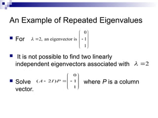
18. An Example of Repeated Eigenvalues
 For
 It is not possible to find two linearly
independent eigenvectors associated with
 Solve where P is a column
vector.
0
2, an eigenvector is 1
1

 
 
 
 
 
 
2
 
0
( 2 ) 1
1
A I P
 
 
  
 
 
 

19. An Example of Repeated Eigenvalues
 With
 P=
 The solution is
 NOTE THE FORM OF THE SOLUTION.
0 1 0 0 0
( 2 ) 1 0 1 1 1
1 0 1 1 1
x
A I P y
z

       
       
     
       
       
 
       
0
1
0
 
 

 
 
 
2 2 2
1 2 3
1 0 0 0
0 1 1 1
0 1 1 0
t t t t
X c e c e c te e
 
       
 
       
      
 
       
       
 
       
 