Downloaded 37 times
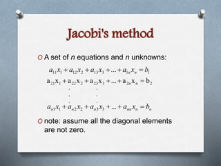
![Jacobi's method
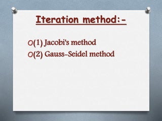
O If diagonal elements are zero then we
Rewrite the question as…
O 푥1 =
[푏1− 푎11푥2+푎13푥3+⋯+푎1푛푥푛 ]
푎11
O 푥2 =
[푏2− 푎21푥2+푎23푥3+⋯+푎2푛푥푛 ]
푎22
O 푥푛 =
[푏푛− 푎푛1푥2+푎푛2푥2+⋯+푎푛(푛−1)푥푛−1 ]
푎푛푛](https://image.slidesharecdn.com/maths-4-141105102701-conversion-gate01/85/system-of-algebraic-equation-by-Iteration-method-5-320.jpg)
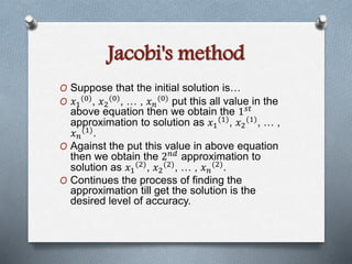
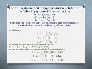
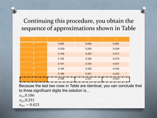
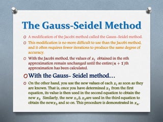
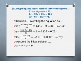
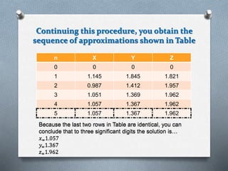
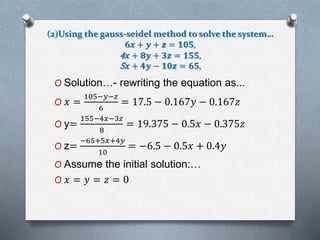
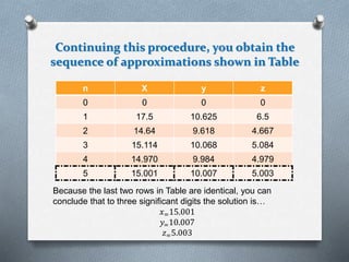
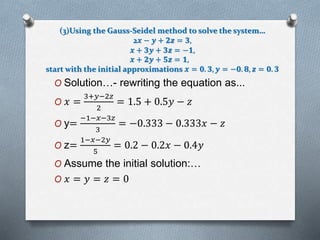
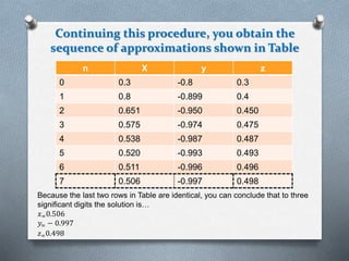
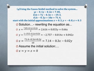
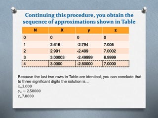


The document discusses iterative methods for solving systems of linear equations, specifically Jacobi's method and Gauss-Seidel method. It provides examples of using these methods to solve several systems of 3 equations with 3 unknowns. For each system, it shows rewriting the equations in a form suitable for the methods, choosing initial approximations, iterating to obtain better approximations, and concluding when subsequent iterations yield identical results to 3 significant digits.