Stability Analysis for Steady State Solutions of Huxley Equation

Raf. J. Of Comp. & Math’s. , Vol. 2, No. 1, 2005
69
Stability Analysis for Steady State Solutions of Huxley Equation
Saad Manaa Mohammad Sabawi
College of Computers Sciences & Mathematics
University of Mosul
Received on: 09/11/2004 Accepted on: 05/04/2005
‫ﺍﻟﻤﻠﺨﺹ‬
‫ﺍﻟ‬ ‫ﺍﻟﺤﻠﻭل‬ ‫ﺍﺴﺘﻘﺭﺍﺭﻴﺔ‬ ‫ﺩﺭﺍﺴﺔ‬ ‫ﺘﻤﺕ‬‫ﻟﻤﻌﺎﺩﻟﺔ‬ ‫ﻼﺯﻤﻨﻴﺔ‬Huxley‫ﺍﻷﺴﺘﻘﺭﺍﺭﻴﺔ‬ ‫ﺘﺤﻠﻴل‬ ‫ﺒﺎﺴﺘﺨﺩﺍﻡ‬
‫ﺍﻟﻨﻤﻁ‬ ‫ﻤﻥ‬Fourier‫ﺍﻟﻤﺘﻐﻴﺭﺓ‬ ‫ﺍﻟﺴﻌﺔ‬ ‫ﺤﺎﻟﺔ‬ ‫ﻓﻲ‬ ‫ﻭﺍﻟﺜﺎﻨﻴﺔ‬ ‫ﺍﻟﺜﺎﺒﺘﺔ‬ ‫ﺍﻟﺴﻌﺔ‬ ‫ﺤﺎﻟﺔ‬ ‫ﻓﻲ‬ ‫ﺍﻷﻭﻟﻰ‬ ‫ﺤﺎﻟﺘﻴﻥ‬ ‫ﻓﻲ‬.
‫ﺍﻟﺤﻠﻴﻥ‬ ‫ﺒﺎﻥ‬ ‫ﺍﻻﺴﺘﻨﺘﺎﺝ‬ ‫ﺘﻡ‬ ‫ﺇﺫ‬01 =u‫ﻭ‬11 =u‫ﺍﻟﺤﻠﻴﻥ‬ ‫ﺒﻴﻨﻤﺎ‬ ‫ﹰ‬‫ﺎ‬‫ﺩﻭﻤ‬ ‫ﻤﺴﺘﻘﺭﺍﻥ‬au =1‫ﻭ‬
( )Xuu 11 =‫ﻤﺸﺭﻭﻁ‬ ‫ﻨﺤﻭ‬ ‫ﻋﻠﻰ‬ ‫ﻤﺴﺘﻘﺭﻴﻥ‬.‫ﺘﻡ‬ ‫ﺍﻟﺘﻲ‬ ‫ﺍﻟﻨﺘﺎﺌﺞ‬ ‫ﺒﻴﻥ‬ ‫ﺍﻟﻤﻘﺎﺭﻨﺔ‬ ‫ﺘﻤﺕ‬ ‫ﺍﻟﺜﺎﻨﻴﺔ‬ ‫ﺍﻟﺤﺎﻟﺔ‬ ‫ﻭﻓﻲ‬
‫ﻁﺭﻴﻘﺔ‬ ‫ﻨﺘﺎﺌﺞ‬ ‫ﻤﻊ‬ ‫ﺍﻟﺘﺤﻠﻴﻠﻲ‬ ‫ﺍﻟﺤل‬ ‫ﻤﻥ‬ ‫ﻋﻠﻴﻬﺎ‬ ‫ﺍﻟﺤﺼﻭل‬Galerkin‫ﻫـﻲ‬ ‫ﺍﻟﻨﺘﺎﺌﺞ‬ ‫ﺇﻥ‬ ‫ﺘﺒﻴﻥ‬ ‫ﻭﻗﺩ‬ ‫ﺍﻟﻌﺩﺩﻴﺔ‬
‫ﺍﻟﺤﺎﻟﺘﻴﻥ‬ ‫ﻜﻠﺘﺎ‬ ‫ﻓﻲ‬ ‫ﻨﻔﺴﻬﺎ‬.
ABSTRACT
Stability analysis of steady state solutions of Huxley equation using
Fourier mode stability analysis in two cases is investigated. Firstly when the
amplitude is constant and secondly when the amplitude is variable and the
results were found to be: The solutions 01 =u and 11 =u are always stable
while the solutions au =1 and ( )Xuu 11 = are conditionally stable. In the
second case, a comparison between the analytical solution and the numerical
solution of Galerkin method is done and the results are the same.

SaadManaa &Mohammad Sabawi
70
1. Introduction
Consider a system of any nature whatsoever that exists in a state S.
We say that S is stable, in one sense or another, if small perturbations or
changes in the system do not drastically affect the state S. For example, the
solar system currently exists in a time-dependent state in which the planets
move about the sun in an orderly fashion. It is known that if a small
additional celestial body is introduced into the system, then the original state
is not disturbed to any significant degree. We say that the original state is
stable to small perturbations. Similar questions of stability arise in every
physical problem (Logan (1987)). McKean (1970) investigated the steady
state solutions of Huxley equation for some values of the wave velocity c.
Maginu (1978) studied by the use of Liapunove’s second method the
stability of such stationary solutions. Fife (1979) analyzed the possible
asymptotic behavior of stationary solutions of bistable equation. Conley and
Smoller (1980) used some topological concepts in the study of stationary
solutions. Smoller and Wasserman (1981) obtained the exact number of
steady state solutions subject to Dirichlet boundary conditions. Manoranjan
et al (1984) obtained the estimates for the critical lengths of the domain at
which bifurcation occurs in the cases 1,)2/10(,0 andaab ≤<= .
Manoranjan (1984) studied in detail the solutions bifurcating from the
equilibrium state au = .
Eilbeck and Manoranjan (1986) considered different types functions
for the pseudo-spectral method applied to the nonlinear reaction-diffusion
equation in 1- and 2- space dimensions. Eilbeck (1986) extended the
pseudo-spectral method to follow steady state solutions as a function of the
problem parameter, using path-following techniques.
Fath and Domanski (1999) studied the cellular differentiation in a
developing organism via a discrete bistable reaction-diffusion model and
they investigated some properties of the bifurcation of steady state solutions.
Lewis and Keener (2000) studied the propagation failure using the one-
dimensional scalar bistable equation by a passive gap and they reduced the
problem of finding conditions for block to the problem of finding the
existence of steady state solutions.
In this paper, the stability of steady state solutions of Huxley equation is
analyzed.

Stability Analysis for Steady…
71
2. The Mathematical Model
One of the famous nonlinear reaction-diffusion equations is the
generalized Burgers-Huxley (gBH) equation:
( )( ) ( )
( )0,1a&0,0,0
112
2
∈>≥≥
−−=
∂
∂
−
∂
∂
+
∂
∂
δβα
βα δδδ
auuu
x
u
x
u
u
t
u
If we take 0,0,1 ≠≠= βαδ and , equation (1) becomes the
following Burgers-Huxley (BH) equation:
( )( ) ( )212
2
auuu
x
u
x
u
u
t
u
−−=
∂
∂
−
∂
∂
+
∂
∂
βα
Equation (2) shows a prototype model for describing the interaction
mechanism, convection transport. When 1,0 == δβ , equation (1) is
reduced to Burgers equation which describes the far field of wave
propagation in nonlinear dissipative systems
( )302
2
=
∂
∂
−
∂
∂
+
∂
∂
x
u
x
u
u
t
u
α
When 1,0 == δα , equation (1) is reduced to the Huxley equation which
describes nerve pulse propagation in nerve fibers and wall motion in liquid
crystals
( )( ) ( )412
2
auuu
x
u
t
u
−−=
∂
∂
−
∂
∂
β
It is known that non-linear diffusion equations (3) and (4) play
important roles in nonlinear physics. They are of special significance for
studying nonlinear phenomena ( Wang et al, 1990). Zeldovich and Frank-
Kamenetsky formulated the equation (4) in 1938 as a model for flame front
propagation and for this reason this equation is sometimes named
Zeldovich-Frank-Kamenetsky (ZF) equation, which has been extensively
studied as a simple nerve model (Binczak et al, 2001). In 1952, Hodgkin
and Huxley proposed their famous Hodgkin-Huxley model for nerve
propagation.
Because of the mathematical complexity of this model, it led to the
introduction of the simpler Fitzhugh-Nagumo system. The simplified model
of the Fitzhugh-Nagumo system is Huxley equation (Wang,1985). Because
Huxley equation is a special case of Fitzhugh-Nagumo system, it is

72
sometimes named Fitzhugh-Nagumo (FN) equation (Estevez and Gordoa,
1990) or the reduced Nagumo equation or Nagumo equation ( Pesin and
Yurchenko, 2004). In sixties, Fitzhugh used equation (4) as an approximate
equation for the description of dynamics of the giant axon. This equation
was among the first models of excited media (Landa,1996).
In this paper, we shall take the Huxley equation as a model problem
(Manoranjan et al ,1984):
( )( )
[ ]
( ) ( )
( ) ( ) ( )5,,
0,0,0,
0,LL,-x
1
2
2
2
btLutLu
HbHxHbxu
t
auuu
x
u
t
u
==−
>≥+−=
≥∈
−−=
∂
∂
−
∂
∂
β
For a dimensionless form, we introduce the following dimensionless
quantities:
2
/,/ LtTLxX ==
Substitute these non-dimensional quantities in equation (4), it follows that:
( )( ) ( )
( ) ( ) ( )71X1-,0b,,1,1
612
2
2
≤≤≥==−
−−+
∂
∂
=
∂
∂
btutu
auuuL
X
u
T
u
β
The equations (6) and (7) represent the non-dimensional form of Huxley
equation in x and t.
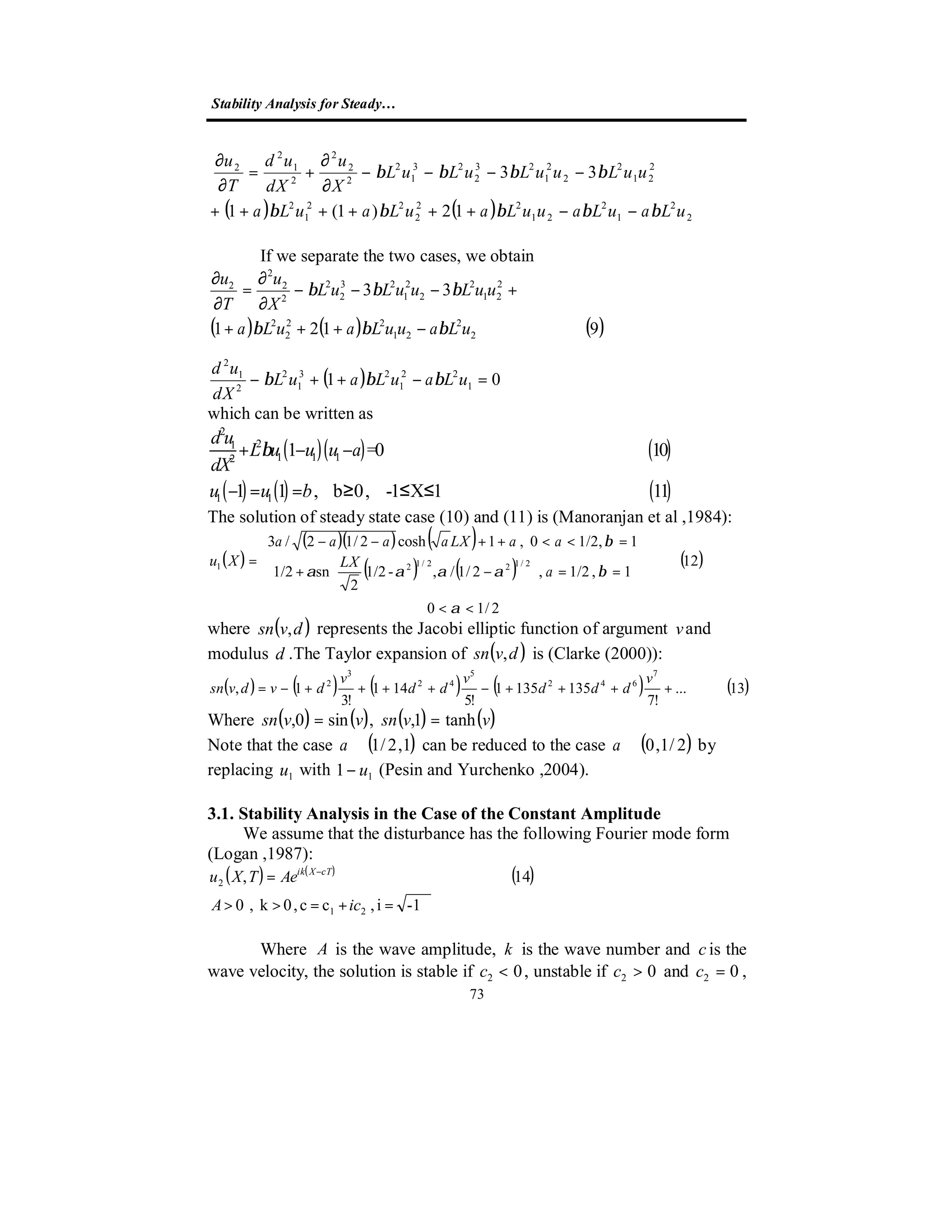
3. Fourier Mode Stability Analysis
Assume that the solution of equation (6) can be written in the form
(Logan ,1987):
( ) ( ) ( ) ( )8,, 21 TXuXuTXu +=
where ( )Xu1 is the steady state solution and ( )TXu ,2 is the disturbance.
Substitute (8) in (6), with its boundary conditions, we get the following
equation:

73
( ) ( )12)1(1
33
2
2
1
2
21
22
2
22
1
2
2
21
2
2
2
1
23
2
23
1
2
2
2
2
2
1
2
2
uLauLauuLauLauLa
uuLuuLuLuL
X
u
dX
ud
T
u
βββββ
ββββ
−−++++++
−−−−
∂
∂
+=
∂
∂
If we separate the two cases, we obtain
( ) ( ) ( )9121
33
2
2
21
22
2
2
2
21
2
2
2
1
23
2
2
2
2
2
2
uLauuLauLa
uuLuuLuL
X
u
T
u
βββ
βββ
−+++
+−−−
∂
∂
=
∂
∂
( ) 01 1
22
1
23
1
2
2
1
2
=−++− uLauLauL
dX
ud
βββ
which can be written as
( )( ) ( )
( ) ( ) ( )
2
21
1 1 12
1 1
1 =0 10
1 1 , b 0, -1 X 1 11
d u
L u u u a
dX
u u b
β+ − −
− = = ≥ ≤ ≤
The solution of steady state case (10) and (11) is (Manoranjan et al ,1984):
( )
( )( ) ( )
( ) ( ) ( )
2/10
12
1,1/2,2/1/,-1/2
2
sn1/2
11/2,0,1cosh2/12/3
2/122/121
<<










==





−+
=<<++−−
=
α
βαααα
β
a
LX
aaLXaaaa
Xu
where ( )dvsn , represents the Jacobi elliptic function of argument vand
modulus d .The Taylor expansion of ( )dvsn , is (Clarke (2000)):
( ) ( ) ( ) ( ) ( )13...
!7
1351351
!5
141
!3
1,
7
642
5
42
3
2
++++−++++−=
v
ddd
v
dd
v
dvdvsn
Where ( ) ( ) ( ) ( )vvsnvvsn tanh1,,sin0, ==
Note that the case ( )1,2/1∈a can be reduced to the case ( )2/1,0∈a by
replacing 1u with 11 u− (Pesin and Yurchenko ,2004).
3.1. Stability Analysis in the Case of the Constant Amplitude
We assume that the disturbance has the following Fourier mode form
(Logan ,1987):
( ) ( )
( )
1-i,cc,0k,0
14,
21
2
=+=>>
= −
icA
AeTXu cTXik
Where A is the wave amplitude, k is the wave number and c is the
wave velocity, the solution is stable if 02 <c , unstable if 02 >c and 02 =c ,

74
gives the neutral stability curve which separate between the stable region
and the unstable region (when 02 <c the disturbance decays as ∞→t and
the stationary solution will be stable, while in the case 02 >c the
disturbance (perturbation) grows as ∞→t and the equilibrium state (rest
point) solution will be unstable, the quantity 2c is called the stability
indicator).
Neglecting the non-linear terms in equation (9), we have:
( ) ( )15123 2
2
21
2
2
2
1
2
2
2
2
2
uLauuLauuL
X
u
T
u
βββ −++−
∂
∂
=
∂
∂
Substitute (14) in (15), we get
( )
k
La
k
uLa
k
uL
kcic
2
1
22
1
2
21
123 βββ
−
+
+−−=+−
Equating the real and imaginary parts, we get
( ) ( ) ( )16
123
0
1
22
1
22
2
1





 +−++
−=
=
k
uLaauLk
c
c
ββ
According to the sign of 2c , we have the following three cases:
, then 02 >c , and the solution ( ) ( ) 1
22
1
22
123 uLaauLk ββ +<++ (i) If
is unstable.
, then 02 <c , and the solution ( ) ( ) 1
22
1
22
123 uLaauLk ββ +>++ (ii) If
is stable.
then 02 =c , which gives ( ) ( ) ,123 1
22
1
22
uLaauLk ββ +=++ (iii) If
the neutral stability curve
( ) ( ) ( )17312 2
1
2
1
2
auLuLak +−+= ββ
( ) ( )auLuLa +>+ 2
1
2
1
2
312 ββIf
Now, we shall apply the results above on the following four cases:
(a) When 01 =u , substitute in (16), we have
0
22
2 <




 +
−=
k
Lak
c
β
i.e. the steady state case 01 =u is always stable.
When 11 =u , substitute in (16), we have (b)
( ) 0
122
2 <




 −+
−=
k
aLk
c
β
(c) When au =1 , substitute in (16), we get

75
( )18
2222
2 




 −+
−=
k
LaLak
c
ββ
From (18), we have
, then02 >c, and the solution is unstable.2222
LaLak ββ <+(i) If
, then,02 <cand the solution is stable.2222
LaLak ββ >+(ii) If
, then02 =c, substitute02 =cin Eq.(18), we get2222
LaLak ββ =+(iii) If
( )
( ) ( )191
10
2
222222222
aLak
aLaLaLakLaLak
−=
⇒−=−=⇒=−+
β
βββββ
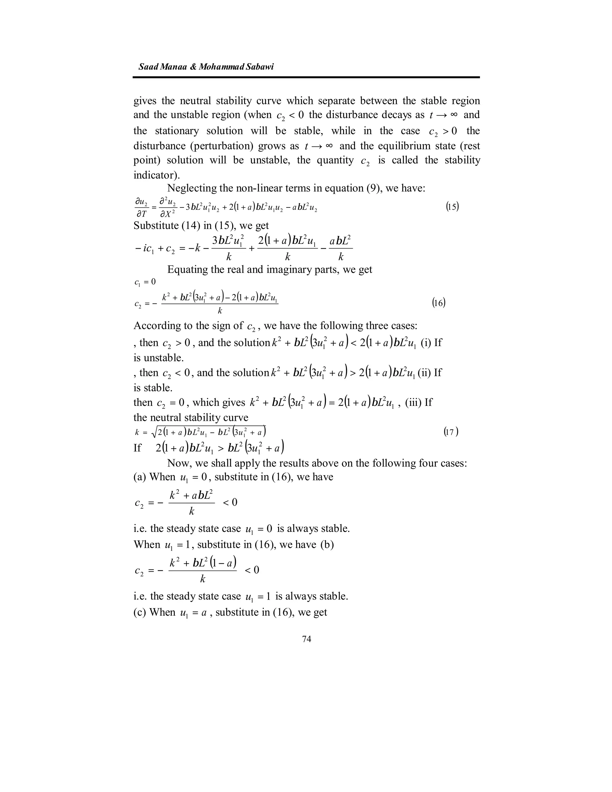
which is the neutral stability curve as in figure (1).
Figure (1) shows the neutral stability curve( )aLak −= 12
βfor the steady
state solutionau =1when9.01.0,1,1 ≤≤== aandLβ
(d) When ( )Xuu 11 = (function of X) as in the equation (12), substitute in
(16), we get
( )( ) ( ) ( )[ ] ( )20/)123( 1
22
1
22
2 kXuLaaXuLkc ββ +−++−=
From (20), we have
(i) If ( )( ) ( ) ( )XuLaaXuLk 1
22
1
22
123 ββ +<++ ,then 02 >c , and the solution
is unstable.
(ii)If ( )( ) ( ) ( )XuLaaXuLk 1
22
1
22
123 ββ +>++ , then ,02 <c and the solution
is stable.
, then,02 =cwhich gives( )( ) ( ) ( )XuLaaXuLk 1
22
1
22
123 ββ +=++(iii) If

76
the neutral stability curve
( ) ( ) ( )( ) ( )21312 2
1
2
1
2
aXuLXuLak +−+= ββ
( ) ( ) ( )( )aXuLXuLa +>+ 2
1
2
1
2
312 ββIf
3.2. Stability Analysis in the Case of the Variable Amplitude
We shall compare the analytical solution with the solution of Galerkin
numerical technique.
3.2.1. The Analytical Solution
We assume that the disturbance case has the following Fourier mode
form (Logan ,1987):
( ) ( ) ( )
( )22,2
CTXik
eXATXu −
=
Substitute (22) in (15) and neglecting the imaginary terms in the
resulting equation, we have
( ) ( )( ) ( ) 0312 2
222
1
2
1
2
=−−−−++′′ XAkckLauLuLaXA βββ
The equation above can be rewritten in the following form:
( ) ( ) ( )
( ) ( ) ( )240b,1X1-,11
230
≥≤≤==−
=+′′
bAA
XDAXA
( ) 2
222
1
2
1
2
312 kckLauLuLaD −−−−+= βββ
The boundary conditions of the amplitude function are the same as
the boundary conditions of the original problem.
The solution of (23) and (24) has the following three cases (Logan
,1987):
(i) If 0<D , then the general solution of (23) and (24) is:
( ) XDXD
eaeaXA −−−
+= 21
Since cosh ( ) / 2x x
x e e−
= + and sinh ( ) / 2x x
x e e−
= −
The solution in above can be written as:
( ) ( )25)sinh()cosh( XDCXDBXA −+−=
Where CB, are arbitrary constants.
Calling the constant D− does not mean that
it is negative, we use the negative sign only for convenience.
From the boundary conditions, we have
( )
bDC
bDCDB
=−+
=−−−
sinhD-Bcosh
26sinhcosh
By adding the two equations in above, we get
DbB −= cosh/
Since 0sinh ≠− D

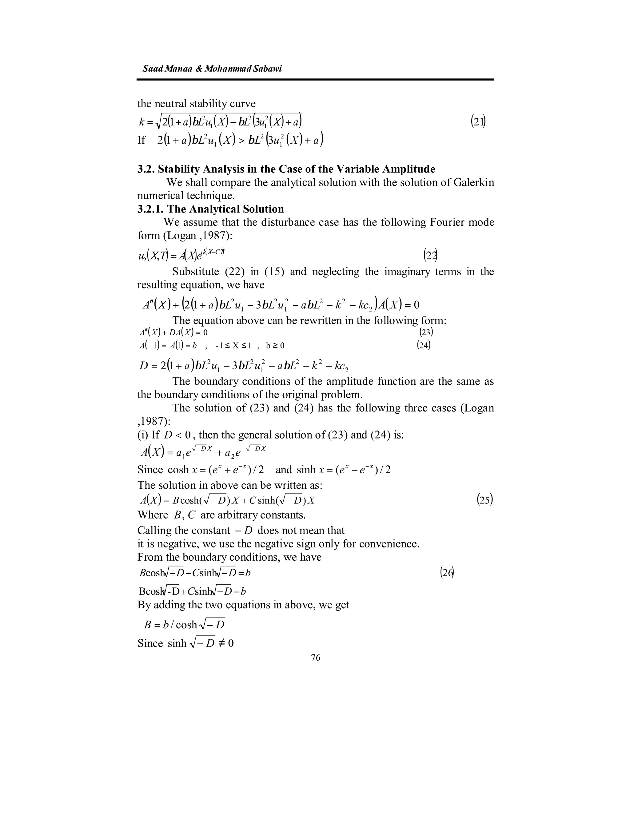
77
substitute Bin one of the two equations above, we have
0sinh ≠− DC . Because 0≠D which implies that 0=C
Substitute B and C in the general solution (25), we get
( ) )27(cosh
cosh
XD
D
b
XA −





−
=
(ii) If 0=D , then the general solution of (23) and (24) is:
( ) ( )28CBXXA +=
( )29



=+
=−
bBC
bBC
By solving the algebraic system (29), we get
bCB == ,0
Substitute Band C in the general solution (28), we get
( ) ( )30bXA =
(iii) If 0>D , then the general solution of (23) and (24) is:
( ) ( )31sincos XDCXDBXA +=
( )32
sinDBcos
sincos




=+
=−
bDC
bDCDB
bB =
( ) ( )33,...3,2,1,
2
== nnD π
Substitute DandB in the general solution (31), we get
( ) ( ) ( ) ( )34sincos XnCXnbXA ππ +=
From (33), we have
( ) ( )[ ] ( )35/)12)3((c 1
22
1
222
2 kuLaauLnk ββπ +−+++−=
Equation (35), has the following three cases:
(i) If ( ) ( ) ( ) 1
22
1
222
123 uLaauLnk ββπ +<+++ , then 02 >c , and the
solution is unstable.
(ii) If ( ) ( ) ( ) 1
22
1
222
123 uLaauLnk ββπ +>+++ , then ,02 <c and the
solution is stable.
(iii) If ( ) ( ) ( ) 1
22
1
222
123 uLaauLnk ββπ +=+++ , then 02 =c , to get the
neutral stability curve, we take the smallest eigenvalue when 1=n

78
( ) ( ) ( )36869604401.9312 2
1
2
1
2
−+−+= auLuLak ββ
( ) ( ) 869604401.9312 2
1
2
1
2
++>+ auLuLa ββIf
The values for which the problem has a nontrivial solution are called
the eigenvalues and the corresponding solutions are called the
eigenfunctions.
According to these results, we have the following three cases:
(a) When 01 =u , substitute in (35), we have
( )[ ] 0/)( 222
2 <++−= kLankc βπ
(b) When 11 =u , substitute in (35), we have
( ) ( )[ ] 0/)1( 222
2 <−++−= kaLnkc βπ
(c) When au =1 , substitute in (35), we get
( )[ ] ( )37/)( 22222
2 kLaLankc ββπ −++−=
From (37), we have
, then02 >c, and the solution is unstable.( ) 22222
LaLank ββπ <++(i) If
, then02 <c, and the solution is stable.( ) 22222
LaLank ββπ >++(ii) If
, then02 =c, to get the neutral stability( ) 22222
LaLank ββπ >++(iii) If
curve , we take the smallest eigenvalue when 1=n
( ) 869604401.912
−−= aLak β
If ( ) 869604401.912
>− aLaβ
(d) When ( )Xuu 11 = (function of X ) as in the equation (12), substitute in
(35), we get
( ) ( )( ) ( ) ( )[ ] ( )38/)123( 1
22
1
222
2 kXuLaaXuLnkc ββπ +−+++−=
From (38), we have
(i) If ( ) ( )( ) ( ) ( ) ,123 1
22
1
222
XuLaaXuLnk ββπ +<+++ then ,02 >c and
the solution is unstable.
(ii) If ( ) ( )( ) ( ) ( )XuLaaXuLnk 1
22
1
222
123 ββπ +>+++ , then 02 <c , and the
solution is stable.
(iii) If ( ) ( )( ) ( ) ( )XuLaaXuLnk 1
22
1
222
123 ββπ +=+++ , then 02 =c , to get
the neutral stability curve , we take the smallest eigenvalue when 1=n
( ) ( ) ( )( ) ( )39869604401.9312 2
1
2
1
2
−+−+= aXuLXuLak ββ

79
If ( ) ( ) ( )( ) 869604401.9312 2
1
2
1
2
++>+ aXuLXuLa ββ
3.2.2. Stability Analysis Using Galerkin Method
The residual methods as Galerkin method usually starts with a
governing boundary value problem. The differential equation is written so
that zero occurs on one side of the equal sign. If the exact solution T could
be substituted into the equation, the result would be zero . The exact
solution is not known, so some approximation of the exact solution TT ≅*
is employed instead. Substitution of the approximate solution into the
differential equation results in an erroneous value r , rather than zero, the
error r is then multiplied by weighting function w, and the product is
integrated over the solution region. The result is called the residual Rand is
set equal to zero (Allaire, 1985).
Let the solution of the equations (23) and (24) be in the form:
( ) ( ) ( )40sincos
1
∑
∞
=
+=
n
nnnn XCXBXA λλ
To find nλ ,we can take any typical term of the summation above as
follows:
( ) XCXBXA nnnn λλ sincos +=
By using the boundary conditions, we have
( )41
sincosB
bsincos
n 


=+
=−
bC
CB
nnn
nnnn
λλ
λλ
( )42,...3,2,1, == nnn πλ
( )43bBn =
Substitute (42) and (43) in (40), we get
( ) ( ) ( )( ) ( )44sincos
1
∑
∞
=
+=
n
n XnCXnbXA ππ
Substitute (44) in (23), we get
( ) ( ) ( ) ( ) ( ) ( )∑ ∑
∞
=
∞
=
=+−+
1 1
22
0)sincos()sincos(
n
n
n
n XnCnXnbnXnCXnbD ππππππ
The residual is:
( )[ ] ( ) ( ) ( )45)sincos(
1
2
RXnCXnbnD n
p
n
=+−∑=
πππ
Using Galerkin assumption (Al-Obaidi and Ibrahim ,2001), we have

80
( )[ ] ( ) ( ) ( )∫ ∑
− =
=





+
1
1
p
1n
2
0dX)sincos(-D XXnCXnbn mn φπππ
( ) (46)1,2,3,....m,,cos m === πλλφ mXX mm
Any element of the matrix will have the form:
( ) ( )[ ] ( ) ( ) ( ) ( )∫∑∑
− = =
+−=
1
1 1 1
2
47cos)sincos(,
p
n
p
m
n dXXmXnCXnbnDmnX ππππ
The following analytical integrals will be useful:
(1) ( ) ( ) 





≠
=
=∫−
mnif
mnif
XdXmXn
0
1
coscos
1
1
ππ
(2) ( ) ( )∫−
=
1
1
,0cossin mnXdXmXn anyforππ
To determine the value of 2c , from (47), we get
( ) 0
2
⇒== πnD
( ) ( )2
2
222
1
2
1
2
312 πβββ nkckLauLuLa =−−−−+
After some mathematical manipulation, one may obtain the algebraic
equation:
( ) ( )[ ] ( )49/12)3(c 1
22
1
222
2 kuLaauLnk ββπ +−+++−=
We observe that equation (49) which is obtained by using Galerkin
method is the same as equation (35) which is obtained from the analytical
solution i.e. the equation (49) will give the same results which are obtained
by using the equation (35) in the cases: ,,1,0 111 auuu === and
( ),11 Xuu = if we use it to compute those results , this indicates the
efficiency and accuracy of the Galerkin method.
The solution of the eigenvalue problem in 2x2 matrix is:
283185307.62,43.14159265 21 ==== πλπλ
The solution in the 4x4 matrix is:
56637061.124,424777961.93
283185307.62,141592654.3
43
21
====
====
πλπλ
πλπλ
To get the neutral stability curve, we put 02 =c in equation (49) and
we take the smallest eigenvalue when 1=n , we have
( ) ( ) ( )50869604401.9312 2
1
2
1
2
−+−+= auLuLak ββ
If ( ) ( ) 869604401.9312 2
1
2
1
2
++>+ auLuLa ββ

81
We note that the equation (50), which is obtained by using Galerkin
method, is the same as equation (36), which is obtained by the use of
analytical solution.
4. Conclusions
We concluded in the constant amplitude case that:
(i) The steady state solution 01 =u is always stable.
(ii) The steady state solution 11 =u is always stable.
(iii) The steady state solution au =1 is stable if:
2222
LaLak ββ >+
The neutral stability curve in this case is:
( )aLak −= 12
β
(iv) The steady state solution ( )Xuu 11 = as in the equation (12), is stable if:
( )( ) ( )XuLaaXuLk 1
22
1
22
)1(23 ββ +>++
( ) ( ) ( )( )
( ) ( ) ( )( )aXuXua
aXuXuLak
+>+
+−+=
2
11
2
2
11
2
3L12
312
If β
β
In the case of variable amplitude the comparison between the analytical
solution and the numerical solution of Galerkin method has been done and
the results are the same in the analytical and numerical solution and the
results were found to be:
(i) The steady state solution 01 =u is always stable.
(ii) The steady state solution 11 =u is always stable.
(iii) The steady state solution au =1 is stable if:
( ) 2222
L Laank ββπ >++
( )
( ) 869604401.91La
869604401.91
2
2
If >−
−−=
a
aLak
β
β
(iv) The steady state solution ( )Xuu 11 = as in the equation (12), is stable if:
( ) ( )( ) ( )XuLaaXuLnk 1
22
1
222
)1(23 ββπ +>+++

82
( ) ( ) ( )( )
( ) ( ) ( )( ) 869604401.93LL12
869604401.9312
2
1
2
1
2
2
1
2
1
2
If ++>+
−+−+=
aXuXua
aXuLXuLak
ββ
ββ
Acknowledgement
The authors would like to thank every person helped to make this paper
come to light.

83
REFERENCES
[1] Allaire, P.E., (1985), Basics of the Finite Element Method, Wm. C.
Brown Publishers.
[2] Al-Obaidi, M.F. and Ibrahim, B.M., (2001), Stability Analysis and
Chaos in a Bend Duct, Raf. J. Sci., Vol. 12, No. 1, pp. 91-99.
[3] Binczak, S., Eilbeck, J.C. and Scott, A.C., (2001), Ephaptic
Coupling of Myelinated Nerve Fibers, Physica D 148 pp. 159-174.
[4] Clarke, F., (2000), The Taylor Series Coefficients of the Jacobi
Elliptic Functions, http://www-maths.swan.ac.uk/staff/fwc.
[5] Conley, C. and Smoller, J., (1980), Topological Techniques in
Reaction-Diffusion Equations, In: Jager, W., Rost, H. and Tautu,
P., Eds., Biological Growth and Spread, Lecture Notes in Biological
Mathematics (Springer, Berlin) 38, pp. 473-483.
[6] Eilbeck, J.C. and Manoranjan, V.S., (1986), A Comparison of Basis
Functions for the Pseudo-Spectral Method for a Model
Reaction-Diffusion Problem, J. Comput. Appl. Math., 15, pp. 371-
378.
[7] Eilbeck, J.C., (1986), The Pseudo-Spectral Method and Path
Following in Reaction-Diffusion Bifurcation Studies, SIAM J. Sci.
Stat.Comput.,Vol. 7, No. 2, pp. 599-610.
[8] Estevez, P.G. and Gordoa, P.R., (1990), Painleve Analysis of the
Generalized Burgers-Huxley Equation, J. Phys. A: Math. Gen.,23,
pp. 4831-4837.
[9] Fath, G. and Domanski, Z, (1999), Avalanche of Bifurcations and
Hysteresis in a Model of Cellular Differentiation, Phys. Rev. E.,
Vol. 60, No. 4, pp. 4604-4609.
[10] Fife, P.C., (1979), Long Time Behavior of Solutions of Bistable
Nonlinear Diffusion Equation, Arch. Rat. Mech. Anal., Vol. 70,
No. 1, pp. 31-46.
[11] Landa, P.S., (1996), Nonlinear Oscillations and Waves in
Dynamical Systems, Kluwer Academic Publishers.
[12] Lewis, T. J. and Keener, J.P., (2000), Wave-Block in Excitable
Media Due to Regions of Depressed Excitability, SIAM J. Appl.
Math., Vol. 61, No.1, pp. 293-316.
[13] Logan, J.D., (1987), Applied Mathematics, John Wiley & Sons.

84
[14] Maginu, K., (1978), Stability of Stationary Solutions of a
Semilinear Parabolic Partial Differential Equation, J.Math. Anal.
Appl. 63, pp. 224-243.
[15] Manoranjan, V.S., Mitchell, A.R., Sleeman, B.D. and Yu, K. P.,
(1984), Bifurcation Studies in Reaction-Diffusion, J. Comput.
Appl. Math., 11, pp. 27-37.
[16] Manoranjan, V.S., (1984), Bifurcation Studies in Reaction-
Diffusion II, J. Comput. Appl. Math., 11, pp. 307-314.
[17] McKean, H.P., (1970), Nagumo’s Equation, Adv. In Math., 4, pp.
209-223.
[18] Pesin, Y. and Yurchenko, A., (2004), Some Physical Models of the
Reaction-Diffusion Equation and Coupled Map Lattices, Russian
Math. Surveys, Vol. 59, No. 3, to appear.
[19] Smoller, J. and Wasserman, A., (1981), Global Bifurcation of
Steady State Solutions, J. Differential Equations, 39, pp. 269-290.
[20] Wang, X.Y., (1985), Nerve Propagation and Wall in Liquid
Crystals,Phys. Lett., Vol. 112 A, No. 8, pp. 402-406.
[21] Wang, X.Y., Zhu, Z.S. and Lu, Y.K., (1990), Solitary Wave
Solutions of the Generalized Burgers-Huxley Equation, J. Phys.
A: Math.Gen., 23, pp. 271-274.

Stability Analysis for Steady State Solutions of Huxley Equation

More Related Content

What's hot

Similar to Stability Analysis for Steady State Solutions of Huxley Equation

More from Mohammad Sabawi Lecturer at Mathematics Department/College of Educations for Women/Tikrit University

Recently uploaded

Stability Analysis for Steady State Solutions of Huxley Equation