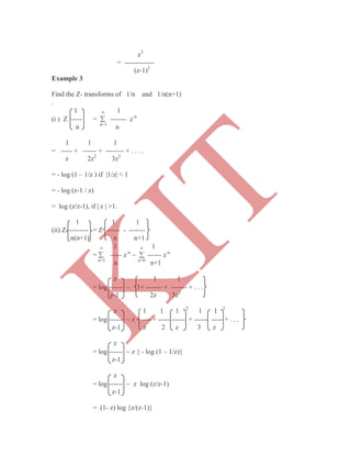
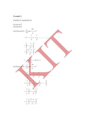
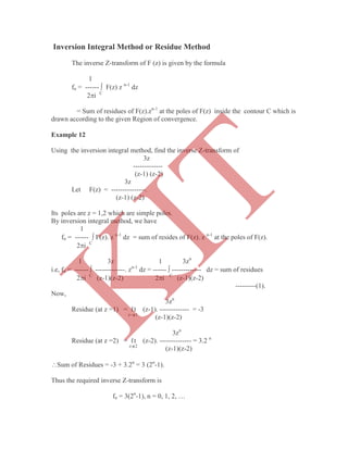
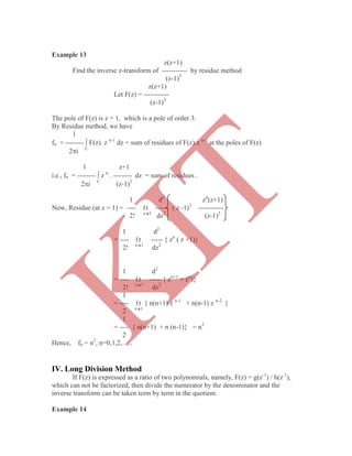
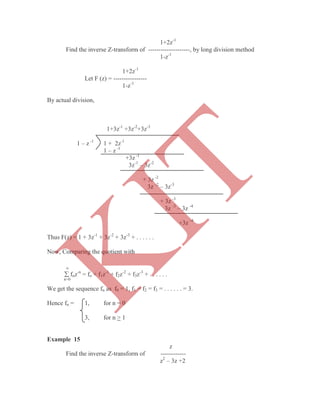
Downloaded 38 times
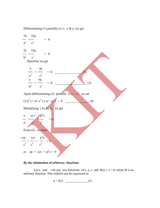
![f (a,b)
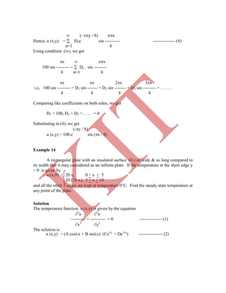
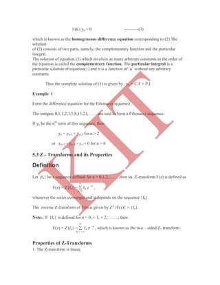
Case (ii) : When F(x,y) = sin(ax + by) (or) cos (ax +by)
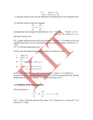
1
P.I = ----------------- sin (ax+by) or cos (ax+by)
f(D2
,DD'
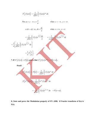
,D'2
)
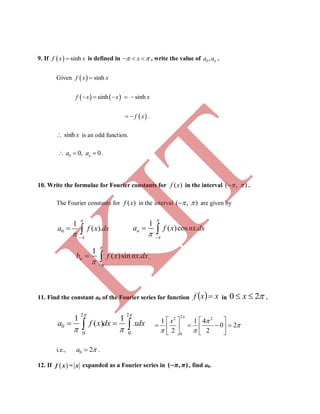
Replacing D2
= -a2
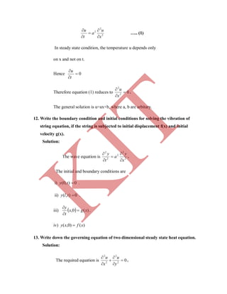
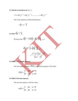
, DD' 2
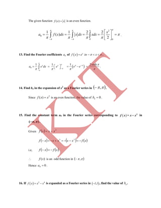
= -ab and D'
= -b2
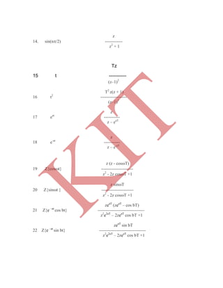
, we get
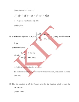
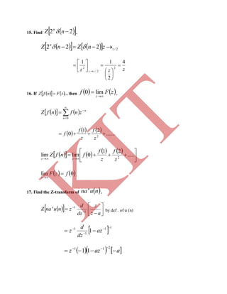
1
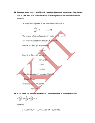
P.I = ----------------- sin (ax+by) or cos (ax+by) , where f(-a2
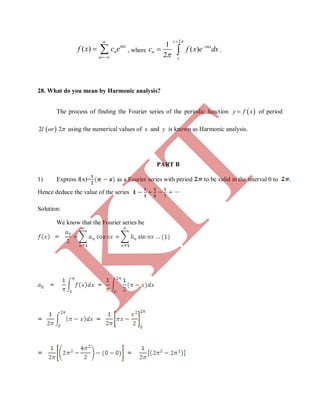
, - ab, -b2
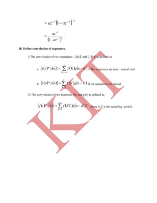
) ≠ 0.
f(-a2
, - ab, -b2
)
Case (iii) : When F(x,y) = xm
yn
,
1
P.I = ---------- xm
yn
= [f (D, D'
)]-1
xm
yn
f(D,D'
)
Expand [f (D,D'
)]-1
in ascending powers of D or D'
and operate on xm
yn
term by term.
Case (iv) : When F(x,y) is any function of x and y.
1
P.I = ---------- F (x,y).
f (D,D'
)
1
Resolve----------- into partial fractions considering f (D,D'
) as a function of D alone.
f (D,D'
)
Then operate each partial fraction on F(x,y) in such a way that
1
--------- F (x,y) = F(x,c-mx) dx ,
D–mD'
where c is replaced by y+mx after integration
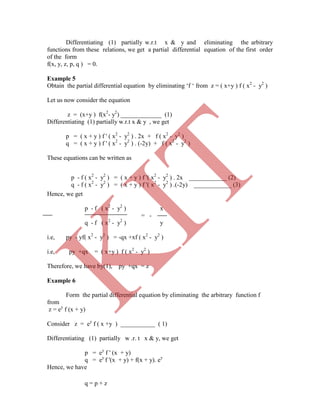
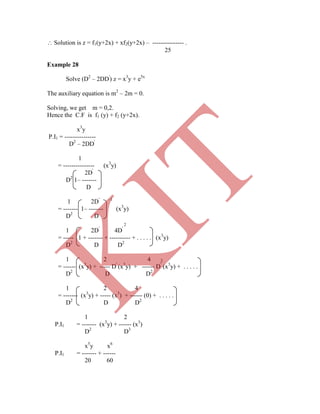
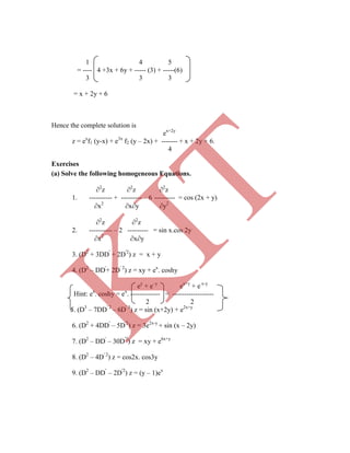
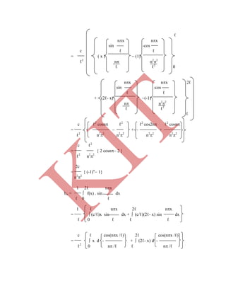
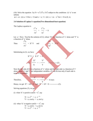
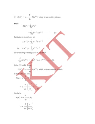
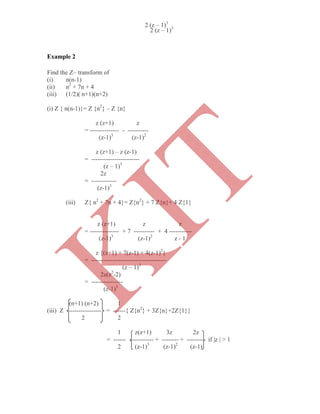
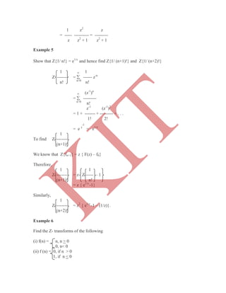
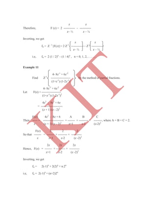
Example 26
Solve(D3
– 3D2
D'
+ 4D'3
) z = ex+2y
The auxillary equation is m=m3
– 3m2
+ 4 = 0
K
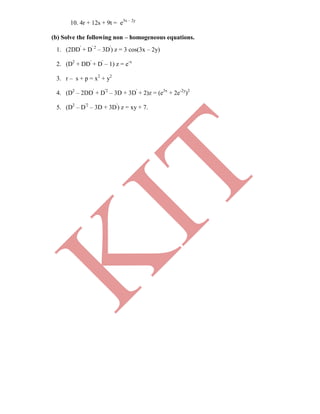
IT](https://image.slidesharecdn.com/mechma6351tpdenotes1-180418083523/85/Mech-MA6351-tpde_notes-33-320.jpg)
![e5x
P.I2 = -------------- (Replace D by 5 and D'
by 0)
D2
– 2DD'
e5x
= ------
25
x5
y x6
e5x
Solution is Z = f1(y) + f2 (y+2x) + ------- + ------ + ------
20 60 25
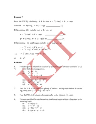
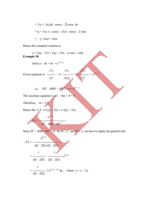
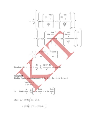
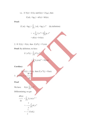
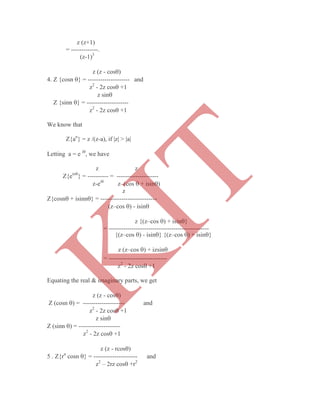
Example 29
2
Solve (D2
+ DD'
– 6 D‟)
z = y cosx.
The auxiliary equation is m2
+ m – 6 = 0.
Therefore, m = –3, 2.
Hence the C.F is f1(y-3x) + f2(y + 2x).
y cosx
P.I = ------------------------
D2
+ DD'
– 6D'
y cosx
= ---------------------------
(D + 3D'
) (D – 2D'
)
1 1
= ------------- --------------- y cosx
(D+3D'
) (D – 2D'
)
1
1
= ------------- (c – 2x) d (sinx)
(D+3D'
)
1
= ------------- [(c – 2x) (sinx) – (-2) ( - cosx)]
(D+3D'
)
1
= ------------- [ y sin x – 2 cos x)]
(D+3D'
)
= [(c + 3x) sinx – 2 cosx] dx , where y = c + 3x
2
= ------------- (c – 2x) cosx dx, where y = c – 2x
(D+3D'
)
K
IT](https://image.slidesharecdn.com/mechma6351tpdenotes1-180418083523/85/Mech-MA6351-tpde_notes-36-320.jpg)
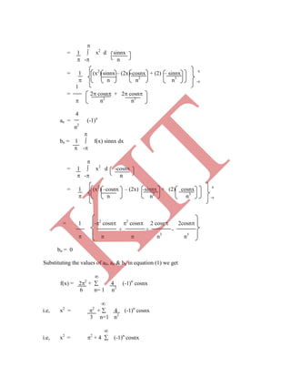
![e2x-y
= --------------
2
e 2x-y
Hence the solution is z = ex
f1 (y+x) + e2x
f2 (y+x) + ----------.
2
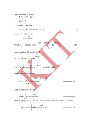
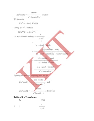
Example 32
Solve (D2
– DD'
+ D'
– 1) z = cos (x + 2y)
The given equation can be rewritten as
(D-D'
+1) (D-1) z = cos (x + 2y)
Here m1 = 1, m2 = 0, c1 = -1, c2 = 1.
Therefore, the C.F = e–x
f1(y+x) + ex
f2 (y)
1 2
P.I = --------------------------- cos (x+2y) [Put D2
= – 1,DD'
= - 2 ,D'
= – 4]
(D2
– DD'
+ D'
– 1)
1
= --------------------------- cos (x+2y)
– 1 – (– 2) + D'
– 1
1
= ------- cos (x+2y)
Hence the solution is z = e-x
f1(y+x) ex
f2(y) + ---------------- .
2
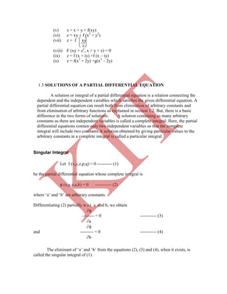
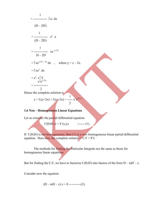
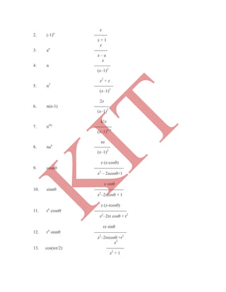
Example 33
Solve [(D + D'
– 1) (D + 2D'
– 3)] z = ex+2y
+ 4 + 3x +6y
Here m1 = – 1, m2 = – 2 , c1 = 1, c2 = 3.
D'
sin (x+2y)
= ----------------
2
sin(x+2y)
K
IT](https://image.slidesharecdn.com/mechma6351tpdenotes1-180418083523/85/Mech-MA6351-tpde_notes-40-320.jpg)
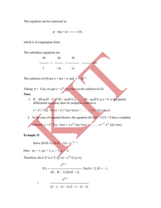
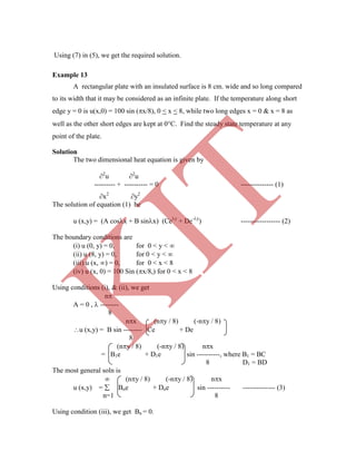
![Hence the C.F is z = ex
f1(y – x) + e3x
f2(y – 2x).
ex+2y
P.I1 = ---------------------------------- [Put D = 1, D'
= 2]
(D+D'
– 1) (D + 2D'
– 3)
ex+2y
= --------------------------
(1+2 – 1) (1+4 – 3)
ex+2y
= ------------
4
1
P.I2 = -------------------------------- (4 + 3x + 6y)
(D+D'
– 1) (D + 2D'
– 3)
1
= --------------------------------------- (4 + 3x + 6y)
D + 2D'
3 [1 – (D+D'
)] 1 – ------------
3
1 D + 2D' -1
= ------ [1 – (D + D'
)]-1
1 – -------------- (4 +3x+6y)
3 3
1 D + 2D'
1
= ----[1 + (D + D'
)+ (D+D'
)2
+ . . .] 1+ ------------- + ----- (D+2D'
)2
+ ….. .]
3 3 9
. (4 + 3x +6y)
1 4 5
= ---- 1 + ----- D + ------D'
+ . . . . . (4 + 3x + 6y)
3 3 3
K
IT](https://image.slidesharecdn.com/mechma6351tpdenotes1-180418083523/85/Mech-MA6351-tpde_notes-41-320.jpg)
![The concept of Fourier series was first introduced by Jacques Fourier (1768–
1830), French Physicist and Mathematician. These series became a most important tool
in Mathematical physics and had deep influence on the further development of
mathematics it self.Fourier series are series of cosines and sines and arise in representing
general periodic functions that occurs in many Science and Engineering problems. Since
the periodic functions are often complicated, it is necessary to express these in terms of
the simple periodic functions of sine and cosine. They play an important role in solving
ordinary and partial differential equations.
A function f (x) is called periodic if it is defined for all real „x‟ and if there is
some positive number „p‟ such that
f (x + p ) = f (x) for all x.
This number „p‟ is called a period of f(x).
If a periodic function f (x) has a smallest period p (>0), this is often called the
fundamental period of f(x). For example, the functions cosx and sinx have fundamental
period 2.
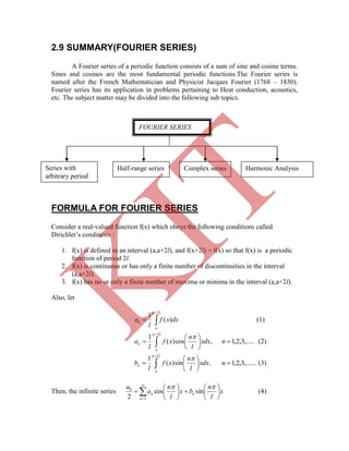
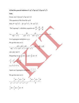
DIRICHLET CONDITIONS
Any function f(x), defined in the interval c x c + 2, can be developed as
a0
a Fourier series of the form ------- + (an cosnx + bn sinnx) provided the following
2 n=1
conditions are satisfied.
f (x) is periodic, single– valued and finite in [ c, c + 2 ].
f (x) has a finite number of discontinuities in [ c, c + 2].
f (x) has at the most a finite number of maxima and minima in [ c,c+ 2].
These conditions are known as Dirichlet conditions. When these conditions are satisfied,
the Fourier series converges to f(x) at every point of continuity. At a point of
discontinuity x = c, the sum of the series is given by
f(x) = (1/2) [ f (c-0) + f (c+0)] ,
UNIT–II
FOURIER SERIES
2.1 INTRODUCTION
2.2 PERIODIC FUNCTIONS
K
IT](https://image.slidesharecdn.com/mechma6351tpdenotes1-180418083523/85/Mech-MA6351-tpde_notes-44-320.jpg)
![where f (c-0) is the limit on the left and f (c+0) is the limit on the right.
EULER’S FORMULAE
The Fourier series for the function f(x) in the interval c < x < c + 2 is given by
a0
f (x) = ------- + (an cosnx + bn sinnx), where
2 n=1
1 C + 2
a0 = ----- f (x) dx.
C
1 C + 2
an = ----- f(x) cosnx dx.
C
1 C + 2
bn = ----- f (x) sinnx dx.
C
= 1 x2
π 2
- π
1 π2
π2
= - = 0
π 2 2
ao = 0
ao ∞
---- + ∑
2 n=1
These values of a0, an, bn are known as Euler‟s formulae. The coefficients a0, an, bn are
also termed as Fourier coefficients.
Example 1
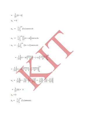
Expand f(x) = x as Fourier Series (Fs) in the interval [ -π, π]
Let f(x) = [ an cos nx + bn sin nx ] ----------(1)
1 π
Here ao = ∫ f (x) dx
π -π
1 π
= ∫ x dx
π -π
π
K
IT](https://image.slidesharecdn.com/mechma6351tpdenotes1-180418083523/85/Mech-MA6351-tpde_notes-45-320.jpg)
![1 π
an = --- ∫ f(x) cosnx dx
π -π
1 π sin nx
= ∫ x d --------
π -π n
π
= 1 (x) sin nx - (1) -cos nx
π n n2
- π
= 1 cos nπ cos nπ
π n2
n2
= 0
1 π
bn = ∫ f(x) sin nx dx
π -π
1 π -cos nx
= ∫ x d n
π -π
1 -cosnx -sin nx π
= (x) - (1)
bn = 2 (-1)n+1
[ cos nπ = (-1)n
]
n
Substituting the values of ao, an & bn in equation (1), we get
π n n2
- π
= 1 - πcos nπ πcosnπ
π n n
= -2π cosnπ
nπ
f(x) = 2(-1)n+1
sin nx
n=1 n
x = 2 sinx - 1 sin2x + 1 sin 3x -……
1 2 3
K
IT](https://image.slidesharecdn.com/mechma6351tpdenotes1-180418083523/85/Mech-MA6351-tpde_notes-46-320.jpg)
![12
22
32
42
12
2. 1 + 1 + 1 + 1 + ………… = 2
12
22
32
42
6
3. 1 + 1 + 1 + 1 + ………… = 2
12
32
52
72
8
Let f(x) = a0 + [ an cosnx + bn sinnx ]
2 n=1
Here
a0 = 1 f(x) dx
-
= 1 x2
dx
-
+
= 1 x3
3 -
= 1 3
3
3 3
ao = 22
3
an = 1 f(x) cosnx dx
-
= 1 x2
cosnx dx
-
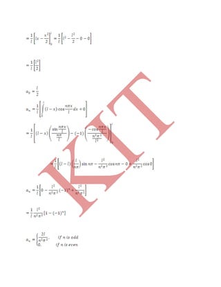
Example 2
Expand f(x) = x2
as a Fourier Series in the interval ( - x ) and hence deduce
that
1. 1 - 1 + 1 - 1 + ………… = 2
K
IT](https://image.slidesharecdn.com/mechma6351tpdenotes1-180418083523/85/Mech-MA6351-tpde_notes-47-320.jpg)
![3 n=1 n2
= 2
+ 4 -cosx + cos2x – cos3x + …..
3 12
22
32
x2
= 2
- 4 cosx + cos2x + cos3x - ….. -----------(2)
3 12
22
32
Put x = 0 in equation (2) we get
0 = 2
- 4 1 – 1 + 1 – 1 + …..
3 12
22
32
42
i.e, 1 – 1 + 1 - …… = 2
-------------(3)
12
22
32
12
Put x = in equation (2) we get
2
= 2
- 4 -1 - 1 - 1 - ………
3 12
22
32
i.e, 2
- 2
= 4 1 + 1 + 1 + ………
3 12
22
32
i.e, 1 + 1 + 1 + …… = 2
-------------(4)
12
22
32
6
Adding equations (3) & (4) we get
1 - 1 + 1 - ….. + 1 + 1 + 1 +…. = 2
+ 2
12
22
32
12
22
32
12 6
i.e, 2 1 + 1 + 1 + ....... = 32
12
32
52
12
i.e, 1 + 1 + 1 + 1 ….. = 2
12
32
52
72
8
Example 3
Obtain the Fourier Series of periodicity 2π for f(x) = ex
in [-π, π]
a0 ∞
Let f(x) = ---- + ∑( an cosnx + bn sinnx) -------------(1)
2 n=1
K
IT](https://image.slidesharecdn.com/mechma6351tpdenotes1-180418083523/85/Mech-MA6351-tpde_notes-49-320.jpg)
![π
a0 = 1 ∫ f(x) dx
π - π
π
= 1 ∫ ex
dx
π - π
π
= 1 [ex
]
π - π
= 2 {eπ
– eπ
}
2π
a0 = 2 sin hπ
π
π
an = 1 ∫ f(x) cos nx dx
π - π
π
= 1 ∫ ex
cos nx dx
π - π
π
= 1 ex
[cosnx + n sin nx]
π (1+n2
) -π
= 1 e π
(-1)n
e π
(-1)n
π 1+n2
1+n2
= (-1)n
( e π
- eπ
)
(1+n2
) π
an = 2 ( -1)n
sin hπ
π(1+n2
)
1 π
bn = ----- ∫ f(x) sin nx dx
π - π
π
= 1 ∫ ex
sin nx dx
π - π
K
IT](https://image.slidesharecdn.com/mechma6351tpdenotes1-180418083523/85/Mech-MA6351-tpde_notes-50-320.jpg)
![1 x2
– (2 - x)2 2
= ----- ------- + --------------
2 0 2
1 2
2
= ------ ------ + ------ =
2 2
i.e, ao =
1 2
an = ----- x cos nx dx + (2 - x) cos nx dx
o
1 sin nx 2 sin nx
= ---- x d --------- + (2 - x) d ---------
0 n
n
o
1 –cos nx 2 –cos nx
= ---- x d --------- + (2 - x) d ---------
o
n
n
1 –cos nx –sinnx
–cos nx – sinnx 2
= ---- (x) --------- – (1) ---------- + (2-x) --------- – (–1) ----------
1 sin nx -cos nx
sin nx – cosnx
= ---- (x) --------- – (1) ---------- + (2-x) --------- – (–1) ----------
n n2
o n n2
1 cos n 1 cos2n cosn
= ---- ----------- – ------- – ------------ + ----------
n2
n2
n2
n2
1 2cos n 2
= ---- ------------ – -------
n2
n2
2
an = -------- [( –1)n
-1]
n2
1 2
bn = ----- f(x) sin nx dx + f(x) sin nx dx
K
IT](https://image.slidesharecdn.com/mechma6351tpdenotes1-180418083523/85/Mech-MA6351-tpde_notes-52-320.jpg)
![ n n2
o n n2
1 – cos n cosn
= ---- -------------- + --------------- = 0
n n
i.e, bn = 0.
2
f (x) = ----- + ------- [ (– 1)n
– 1] cos nx
2 n=1
n2
4 cosx cos3x cos5x
= ----- – ------ -------------- +----------- +------------ + . . . . . -----(2)
2 12
32
52
Putting x = 0 in equation(2), we get
4 1 1 1
0 = ------- – ------- ------ + ------ + ------ + . . . . .
2 12
32
52
1 1 1 2
i.e, ------ + ------ + ------ + . . . . . = -------
12
32
52
8
1 2
i.e, ------------- = -------
n=1
(2n – 1)2
8
Example 5
Find the Fourier series for f (x) = (x + x2
) in (- < x < ) of percodicity 2 and hence
deduce that (1/ n2
) = 2
/6.
n=1
a0
Let f(x) = ------- + ( an cosnx + bn sinnx)
2 n=1
1
Here, a0 = ------ (x + x2
) dx
–
1 x2
x3
= ----- ----- +-----
2 2 3 0
K
IT](https://image.slidesharecdn.com/mechma6351tpdenotes1-180418083523/85/Mech-MA6351-tpde_notes-53-320.jpg)
![ 1 2
Hence, ----- = -------.
n=1
n2
6
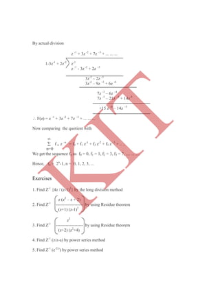
Exercises:
Determine the Fourier expressions of the following functions in the given interval
1.f(x) = ( - x)2
, 0 < x < 2
2.f(x) = 0 in - < x < 0
= in 0 < x <
3.f(x) = x – x2
in [-,]
4.f(x) = x(2-x) in (0,2)
5.f(x) = sinh ax in [-, ]
6.f(x) = cosh ax in [-, ]
7.f(x) = 1 in 0 < x <
= 2 in < x < 2
8.f(x) = -/4 when - < x < 0
= /4 when 0 < x <
9.f(x) = cosx, in - < x < , where „‟ is not an integer
10.Obtain a fourier series to represent e-ax
from x = - to x = . Hence derive the series
for / sinh
x cos x,. are odd functions.
(1) The Euler‟s formula for even function is
a0
f (x) = ------ + an consnx
2 n=1
2 2
where ao = ---- f(x) dx ; an = ----- f (x) cosnx dx
0
0
A function f(x) is said to be even if f (-x) = f (x). For example x2
, cosx, x sinx, secx are
even functions. A function f (x) is said to be odd if f (-x) = - f (x). For example, x3
, sin x,
2.3 Even and Odd functions
K
IT](https://image.slidesharecdn.com/mechma6351tpdenotes1-180418083523/85/Mech-MA6351-tpde_notes-56-320.jpg)
![Expand f (x) = |x| in (-, ) as FS and hence deduce that
1 1 1 2
------ + ----- + ------ . . . . . =. --------
12
32
52
8
Solution
Here f(x) = |x| is an even function.
ao
f (x) = -------- + an cos nx ------- (1)
2 n=1
2
ao = ----- f(x) dx
0
2
= ----- x dx
0
2 x2
= ----- ----- =
2 0
2
an = ----- f (x) cos nx dx
0
2 sin nx
= ----- x d ----------
0
n
2 sin nx – cos nx
= ----- (x) ---------- – (1) -----------
n n2
0
2 cos n 1
= ----- ---------- – ------
n2
n2
2
an = ----- [(– 1) n
– 1]
n2
2
f (x)= -------+ ------- [(–1)n
– 1] cos nx
2 n=1
n2
4 cos x cos3x cos5x
K
IT](https://image.slidesharecdn.com/mechma6351tpdenotes1-180418083523/85/Mech-MA6351-tpde_notes-58-320.jpg)
![2 2x
an = ----- 1 – ------- cos nx dx
0
2 2x sin nx
= ----- 1 – -------- d -----------
0
n
2 2x sin nx – 2 – cosnx
= ----- 1 – ------ --------- – ------- ----------
n n2 0
4
an = ------- [(1– (– 1)n
]
2
n2
4
1 2
or ----------- = --------
n=1
(2n–1)2
8
Example 9
Obtain the FS expansion of f(x) = x sinx in (- < x<) and hence deduce that
1 1 1 - 2
------ – ------- + ------- – . . . . . = ---------
1.3 3.5 5.7 4.
f (x)= -------- [1– (– 1)n
]cos nx
n=1
2
n2
4 2cos x 2cos3x 2cos5x
= ----- ----------- + ---------- + ------------ + . . . . . . -----------(2)
2
12
32
52
Put x = 0 in equation (2) we get
2
1 1 1
------- = 2 ------ + ------- + --------+ . . . . . . .
4 12
32
52
1 1 1 2
==> ------ + ------ + ------ + … = -------
12
32
52
8
K
IT](https://image.slidesharecdn.com/mechma6351tpdenotes1-180418083523/85/Mech-MA6351-tpde_notes-60-320.jpg)
![Here f (x) = xsinx is an even function.
ao
Let f (x) = -------- + an cos nx ------------- (1)
2 n=1
2
Now, ao = ----- xsin x dx
0
2
= ----- x d ( - cosx)
0
2
= ----- (x) (- cosx) – (1) (- sin x)
0
a0 = 2
2
an = ----- f (x) cos nx dx
0
2
= ----- x sin x cosnx dx
0
1
= ----- x [ sin (1+n)x + sin (1 – n)x] dx
0
1 – cos (1+n)x cos (1 – n) x
= ------ x d --------------- – -------------------
0
1 + n 1 – n
1 – cos (1+n)x cos (1 – n) x – sin (1+n)x sin (1 – n) x
= ------ (x) --------------- – --------------- – (1) --------------- – -----------------
1 + n 1 – n (1 + n)2
(1 – n)2
0
1 – cos (1+n) cos (1 – n)
= ------ ------------------- – -------------------
1 + n 1 – n
- [cos cosn - sin sinn] [cos cosn - sin sin n ]
K
IT](https://image.slidesharecdn.com/mechma6351tpdenotes1-180418083523/85/Mech-MA6351-tpde_notes-61-320.jpg)
![where a0 = ------- f(x) dx and
0
2
an = ------- f(x) cosnx dx
0
(ii) Half Range Sine Series
The Fourier sine series for f(x) in the interval (0,) is given by
f(x) = bn sinnx
n=1
2
where bn = ------- f(x) sinnx dx
0
Example 10
If c is the constant in ( 0 < x < ) then show that
c = (4c / ) { sinx + (sin3x /3) + sin5x / 5) + ... ... ... }
Given f(x) = c in (0,).
Let f(x) = bn sinnx (1)
n = 1
2
bn = ------- f(x) sin nx dx
0
2
= ------- c sin nx dx
0
2c - cosnx
= ------- -------------
n 0
2c -(-1)n
1
= ---- ------ + ----
n n
bn = (2c/n) [ 1 – (-1)n
]
K
IT](https://image.slidesharecdn.com/mechma6351tpdenotes1-180418083523/85/Mech-MA6351-tpde_notes-64-320.jpg)
![2
= ------- xdx
0
2 x2
= ------- --- =
2 0
2
an = ------- f(x) cosnx dx
0
2
an = ------- x d (sinnx / n )
0
2
f(x) = --- + ----- [ (-1)n
- 1] cosnx
2 n=1 n2
4 cosx cos3x cos5x
=> x = --- + --- ---------- + ---------- + --------- …… …
2 12
32
52
Example 12
Find the sine and cosine half-range series for the function function .
f(x) = x , 0 < x π/2
= π-x, π/2x<
Sine series
Let f (x) = bn sin nx.
n=1
2 sinnx - cosnx
= ---- (x) ----------- - (1) --------------
n n2
0
2
an = ------ (-1)n
-1
n2
K
IT](https://image.slidesharecdn.com/mechma6351tpdenotes1-180418083523/85/Mech-MA6351-tpde_notes-66-320.jpg)
![∫ [f(x)]2
dx
[f (x)] r m s = a
b – a
The use of r.m.s value of a periodic function is frequently made in the
theory of mechanical vibrations and in electric circuit theory. The r.m.s value is
also known as the effective value of the function.
Parseval’s Theorem
If f(x) defined in the interval (c, c+2π ), then the Parseval‟s Identity is given by
c+2π
∫ [f (x)]2
dx = (Range)
c
or
= ( 2π)
Example 13
Obtain the Fourier series for f(x) = x2
in – π < x < π
Hence show that 1 + 1 + 1 + . . . π4
14
24
34
90
2π2
4 (-1)n
we have ao = 3 , an = n2
, bn = 0, for all n (Refer Example 2).
By Parseval‟s Theorem, we have
π ao2
∞
ao2
1
+ ∑ ( an
2
+ bn
2
)
4 2
ao2
1
+ ∑ ( an
2
+ bn
2
)
4 2
=
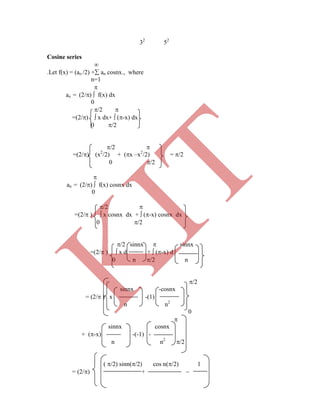
10.Obtain cosine series for
f(x) = cos x , 0<x< (/2)
= 0, /2 < x < .
2.5 Parseval’s Theorem
Root Mean square value of the function f(x) over an interval (a, b) is defined as
b
K
IT](https://image.slidesharecdn.com/mechma6351tpdenotes1-180418083523/85/Mech-MA6351-tpde_notes-70-320.jpg)
![∫ [ f(x)]2
dx = 2π + ½ ∑ (an
2
+ bn
2
)
- π 4 n=1
π 4π4
∞ 16(-1) 2n
i.e, ∫ x4
dx = 2π + 1/2 ∑
- π 36 n=1
n4
π π4
∞ 1
i.e, x5
= 2π + 8 ∑
5 -π 9 n=1
n4
π4
π4
∞ 1
= + 8 ∑
5 9 n=1
n4
∞ 1 π4
=> ∑ =
n=1
n4
90
Hence 1 + 1 + 1 + . . . π4
14
24
34
90
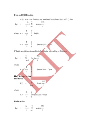
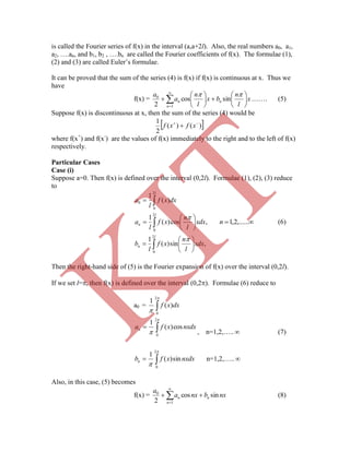
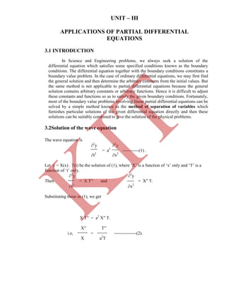
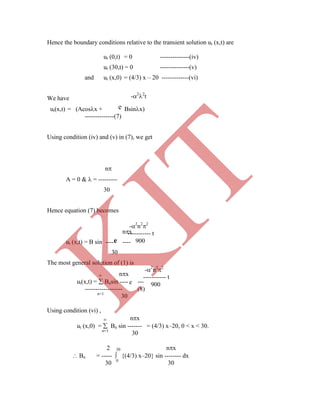
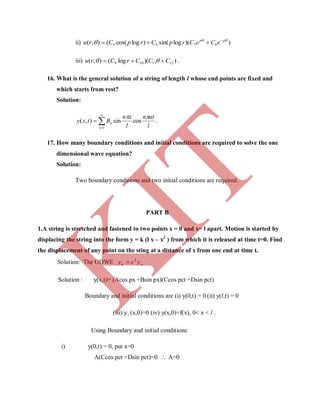
Suppose f(x) is a function defined in the interval c< x < c+2l. The Fourier
expansion for f(x) in the interval c<x<c+2l is given by
a0 nx nx
f(x) = ----- + an cos ---- + bn sin ----
2 n=1 l l
1 c+2 l
where a0 = ----- f(x)dx
l c
1 c+2 l
an = ----- f(x) cos (nx / l ) dx &
l c
1 c+2 l
bn = ----- f(x) sin (nx / l ) dx
l c
=
2.6 CHANGE OF INTERVAL
In most of the Engineering applications, we require an expansion of a given
function over an interval 2l other than 2.
K
IT](https://image.slidesharecdn.com/mechma6351tpdenotes1-180418083523/85/Mech-MA6351-tpde_notes-71-320.jpg)
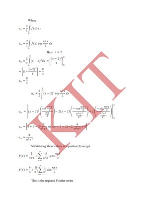
![12.Find the half –range cosine series for the function f(x) = (x-2)2
in the interval
0 < x < 2.
1 2
Deduce that -------- = -----
In (1), the term (a1cosx + b1 sinx) is called the fundamental or first harmonic,
the term (a2cos2x + b2sin2x) is called the second harmonic and so on.
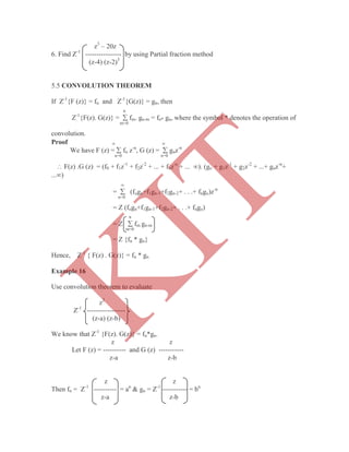
Example 16
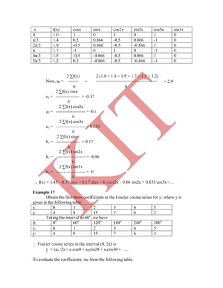
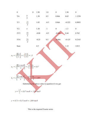
Compute the first three harmonics of the Fourier series of f(x) given by the
following table.
x: 0 π/3 2π/3 π 4π/3 5π/3 2π
f(x): 1.0 1.4 1.9 1.7 1.5 1.2 1.0
We exclude the last point x = 2π.
Let f(x) = (a0/2) + (a1 cosx + b1 sinx) + (a2 cos2x + b2 sin2x) + …………
To evaluate the coefficients, we form the following table.
2 n=1
ie, f(x) = (a0/2) + (a1 cosx + b1 sinx) + (a2 cos2x + b2 sin2x) +
(a3cos3x + b3sin3x)+… -------------(1)
2 ∑ f(x)
Here a0 = 2 [mean values of f(x)] = -----------
n
2 ∑ f(x) cosnx
an = 2 [mean values of f(x) cosnx] = ---------------------
n
2 ∑ f(x) sinnx
& bn = 2 [mean values of f(x) sinnx] = -------------------
n
1 (2n – 1)2
8
2.7 Harmonic Analysis
The process of finding the Fourier series for a function given by numerical values
is known as harmonic analysis.
a0
f (x) = ------- + (an cosnx + bn sinnx), where
K
IT](https://image.slidesharecdn.com/mechma6351tpdenotes1-180418083523/85/Mech-MA6351-tpde_notes-78-320.jpg)

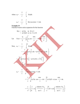
![Example 19
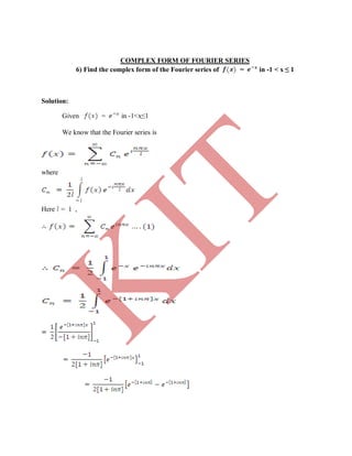
Find the complex form of the Fourier series f(x) = e –x
in -1 ≤ x ≤ 1.
∞ i n π x
We have f(x) = ∑ cn e
n=-∞
l - i n π x
where cn = 1 ∫ e –x
e dx
2 -1
1 - (1+ i n π) x
cn = 1 ∫ e dx
2 -1
= 1 e - (1+i nπ) x 1
2 - (1+inπ) -1
= 1 .
-2 ( 1+inπ ) e - (1 + i n π) x
-e (1+ i nπ)
= (1-inπ) [ e-1
( cos nπ – isin nπ) - e (cos nπ + i sin nπ) ]
-2 ( 1+n2
π2
)
= (1-inπ) cos nπ ( e-1
- e )
-2 ( 1+n2
π2
)
(1-inπ)
Cn = ----------- (-1)n
sinh1
f(x) = ∑ ----------- (-1)n
sinh1 e
n= - ∞ (1+n2
π2
)
Example 20
Find the complex form of the Fourier series f(x) = ex
in - π < x < π.
∞
We have f(x) = ∑ Cn e i nx
n=-∞
1 π
where Cn = ------ ∫ f(x) e – i nx
dx
2π - π
(1+n2
π2
)
∞ (1-inπ) i n π x
K
IT](https://image.slidesharecdn.com/mechma6351tpdenotes1-180418083523/85/Mech-MA6351-tpde_notes-83-320.jpg)
![1 π
= ------ ∫ ex
e –i nx
dx
2π - π
1 π
= ------- ∫ e (1-i n) x
dx
2π - π
π
1 e (1-in)x
= 2π ( 1-in)
-π
= 1 [ e(1-in)π
-e - (1-i n) π
]
2π(1-in)
(1+in)
= ----------- [ eπ
( cos nπ – i sin nπ ) –e -π
( cosn π + i sin nπ)]
2π(1+n)2
(1+in) (-1)n
. e π
– e-π
= ------------- -----------
( 1+n2
) 2π
(-1)n
(1+in) sin h π
= --------------------------
( 1+n2
) π
∞ (-1)n
(1+in) sin h π
f(x) = ∑ ----------------------- e i nx
n= - ∞ ( 1+n2
) π
Exercises
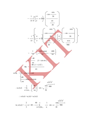
Find the complex form of the Fourier series of the following functions.
1.f(x) = eax
, -l < x < l.
2.f(x) = cosax, - < x < .
3.f(x) = sinx, 0 < x < .
4.f(x) = e-x
, -1 < x < 1.
5.f(x) = sinax, a is not an integer in (-, ).
K
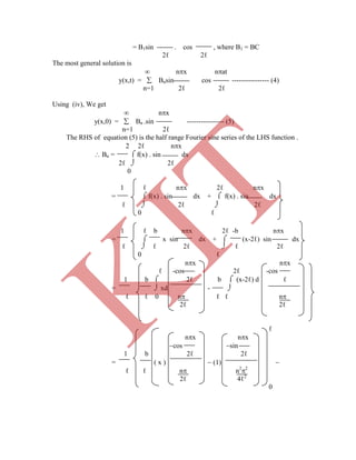
IT](https://image.slidesharecdn.com/mechma6351tpdenotes1-180418083523/85/Mech-MA6351-tpde_notes-84-320.jpg)
![b
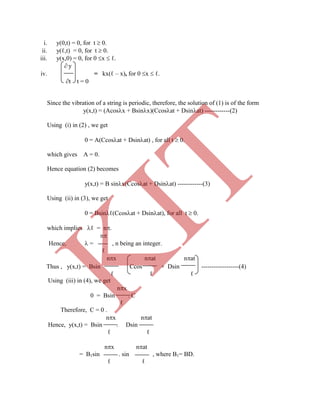
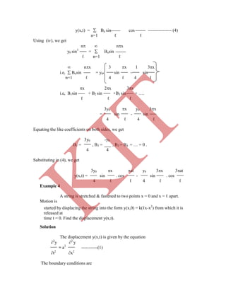
O(0,0) ℓ B(2ℓ,0) x
(b/ℓ)x , 0<x<ℓ
(iv) y(x,0) =
-(b/ℓ)(x-2ℓ), ℓ<x<2ℓ
[Since, equation of OA is y = (b/ℓ)x and equation of AB is (y-b)/(o-b) = (x-ℓ)/(2ℓ-ℓ)]
Using conditions (i) and (ii) in (2), we get
n
A = 0 & =
2ℓ
nx nat nat
y(x,t) = B sin (Ccos + Dsin ) -----------(3)
2ℓ 2ℓ 2ℓ
y nx nat na nat na
Now, = B sin - Csin . + Dcos .
t 2ℓ 2ℓ 2ℓ 2ℓ 2ℓ
Using (iii) in the above equation , we get
nx na
0 = B sin D
2ℓ 2ℓ
Here B can not be zero, therefore D = 0.
Hence equation (3) becomes
nx nat
y(x,t) = B sin . Ccos
2ℓ 2ℓ
nx nat
K
IT](https://image.slidesharecdn.com/mechma6351tpdenotes1-180418083523/85/Mech-MA6351-tpde_notes-102-320.jpg)
![ nx
u (x,0) = Dn. sin --------- ------------ (5)
n =1 10
The RHS of equation (5) is a half range Fourier sine series of the LHS function
2 10 nx
Dn = -------- f (x) sin -------- dx
10 0
10
2 10 10
= ------ (20x) ------------------- – (20) ----------------------
10 n n2
2
-------- -------
10 100 0
nx nx 10
- cos ---------- - sin ----------
n
800 sin --------
2
i.e, Dn = -------------------------
n2
2
Substituting in (4) we get,
n
800 sin --------
2 (-ny / 10) nx
u (x,y) = ------------------------- e sin ----------
n =1
n2
2
10
Example 15
A rectangular plate is bounded by the lines x = 0, x = a, y = 0 & y = b.
The edge temperatures are u (0,y) = 0, u (x,b) = 0, u (a,y) = 0 &
nx nx 5
- cos ---------- - sin ----------
10 10
+ [20 (10–x)] ------------------- – (-20) ----------------------
n n2
2
-------- -------
10 100 5
K
IT](https://image.slidesharecdn.com/mechma6351tpdenotes1-180418083523/85/Mech-MA6351-tpde_notes-129-320.jpg)

![Since, 1 ℓ 1 ℓ
----- f(t) dt ----- f(t) dt ,
2ℓ -ℓ 2ℓ -ℓ
then by assumption (ii), the first term on the right side of (2) approaches zero as ℓ .
As ℓ , the second term on the right side of (2) becomes
1 n(t – x)
ℓim --- f(t) cos ----------- dt
ℓ ℓ n=1 - ℓ
1
= ℓim --- f(t) cos { n (t – x) } dt ,on taking (∕ℓ) =
.
0 n=1 -
By the definition of integral as the limit of sum and (n∕ℓ ) = as ℓ , the second
term of (2) takes the form
1
--- f(t) cos (t – x) dt d ,
0 -
Hence as ℓ , (2) becomes
1
f(x) = --- f(t) cos (t – x) dt d ---------(3)
0 -
which is known as the Fourier integral of f(x).
Note:
f(x) = --- f(t) cos (t – x) dt d
0 -
1
= --- f(t) { cost . cosx + sint . sinx } dt d
0 -
1 1
When f(x) satisfies the conditions stated above, equation (3) holds good at a point
of continuity. But at a point of discontinuity, the value of the integral is (1/ 2) [f(x+0) +
f(x-0)] as in the case of Fourier series.
Fourier sine and cosine Integrals
The Fourier integral of f(x) is given by
1
K
IT](https://image.slidesharecdn.com/mechma6351tpdenotes1-180418083523/85/Mech-MA6351-tpde_notes-137-320.jpg)
![
Then, F{f(-x)} = F(s), where bar denotes complex conjugate.
Proof
1
F(s) = f(x) e-isx
dx .
2 -
Putting x = -t, we get
1
F(s) = f(-t) eisx
dt .
2 -
x
Let g(x) = f(x) dx .
a
Then, g‟(x) = f(x). ------------( i )
Now f [g„(x)] = (-is) G(s), by property (6).
= (-is). F{g(x)}
x
= (-is). F f(x) dx .
a
x
i.e, F{g‟(x)} = (-is). F f(x) dx .
a
x 1
i.e, F f(x) dx = . F{g‟(x)}.
a (-is)
1
= F{f (x)}. [ by ( i )]
(-is)
x F(s)
Thus, F f(x) dx = .
a (-is)
Property (8)
If F(s) is the complex Fourier transform of f(x),
K
IT](https://image.slidesharecdn.com/mechma6351tpdenotes1-180418083523/85/Mech-MA6351-tpde_notes-145-320.jpg)
![1 a eisx
= x .d
2 -a is
a
1 xeisx
eisx
= -
2 is (is)2
-a
1 aeisa
eisa
ae-isa
e-isa
= - + +
2 is (is)2
is (is)2
1 a 1
= (eisa
+ e-isa
) + (eisa
- e-isa
)
2 is s2
1 -2ai 2i
= cossa + sinsa
2 s s2
2i 1
= . [sinsa - as cossa].
s2
2
i [sinsa - as cossa]
= (2/)
s2
Example 3
Find the F.T of f(x) = eiax
, 0 < x < 1
= 0 otherwise
The F.T of f(x) is given by
1
F{f (x)} = eisx
f (x) dx.
2 -
1 1
= eisx
. eiax
dx.
K
IT](https://image.slidesharecdn.com/mechma6351tpdenotes1-180418083523/85/Mech-MA6351-tpde_notes-147-320.jpg)
![2 0
1 1
= ei(s+a)x
.dx .
2 0
1 ei(s+a)x
1
=
2 i(s+a) 0
1
= {ei(s+a)x
-1}
i2.(s+a)
i
= {1- ei(s+a)
}
2.(s+a)
Example 4
2 2 2 2
Find the F.T of e-a x
, a>0 and hence deduce that the F.T of e-x / 2
is e-s / 2
.
The F.T of f(x) is given by
1
F{f (x)} = eisx
f (x) dx.
2 -
2 2 1 2 2
e-s / 4a
2
= e-[ax – (is/2a)]
dx .
2 -
2 2
e-s / 4a
2
= e-t
dt, by putting ax –(is/2a) = t
a2 -
2 2
e-s / 4a
2
= . , since e-t
dt = (using Gamma functions).
a2 -
F e-a x
= e –a x
. eisx
.dx.
2 -
2 2
K
IT](https://image.slidesharecdn.com/mechma6351tpdenotes1-180418083523/85/Mech-MA6351-tpde_notes-148-320.jpg)
![The function Fs(s), as defined by (1), is known as the Fourier sine transform of f(x).
Also the function f(x), as given by (2),is called the Inverse Fourier sine transform of
Fs(s) .
Fourier cosine transform
Similarly, it follows from the Fourier cosine integral
2
f(x) = cos x . f(t) cost dt.d.
0 0
that if Fc(s) = (2/ ) f(x) cossx dx. ------------(3)
0
then f(x) = (2/ ) Fc(s) cossx ds. ------------(4)
0
The function Fc(s), as defined by (3), is known as the Fourier cosine transform of
f(x). Also the function f(x), as given by (4),is called the Inverse Fourier cosine
transform of Fc(s) .
Properties of Fourier sine and cosine Transforms
If Fs(s) and Fc(s) are the Fourier sine and cosine transforms of f(x) respectively, the
following properties and identities are true.
(1) Linearity property
Fs [a f(x) + b g(x) ] = a Fs { f(x) } + b Fs { g(x) }.
and Fc [a f(x) + b g(x) ] = a Fc { f(x) } + b Fc { g(x) }.
(2) Change of scale property
Fs [ f(ax) ] = (1/a) Fs [ s/a ].
and Fc [ f(ax) ] = (1/a) Fc [ s/a ].
(3) Modulation Theorem
i. Fs [ f(x) sinax ] = (1/2) [ Fc (s-a) - Fc (s+a)].
ii. Fs [ f(x) cosax ] = (1/2) [ Fs (s+a) + Fs (s-a)].
K
IT](https://image.slidesharecdn.com/mechma6351tpdenotes1-180418083523/85/Mech-MA6351-tpde_notes-157-320.jpg)
![iii. Fc[ f(x) cosax ] = (1/2) [ Fc (s+a) + Fc (s-a) ].
iv. Fc[ f(x) sinax ] = (1/2) [ Fs (s+a) - Fs (s-a) ].
Proof
The Fourier sine transform of f(x)sinax is given by
Fs [ f(x) sinax ] =(2/ ) (f(x) sinax) sinsx dx.
0
= (1/2) (2/ ) f(x) [cos(s-a)x – cos(s+a)x] dx.
0
= (1/2) [ Fc (s-a) – Fc (s+a) ].
Similarly, we can prove the results (ii), (iii) & (iv).
(4) Parseval’s identity
Fc(s) Gc(s) ds = f(x) g(x) dx .
0 0
Fs(s) Gs(s) ds = f(x) g(x) dx .
0 0
Fc(s) 2
ds = f(x) 2
dx .
0 0
Fs(s) 2
ds = f(x) 2
dx .
0 0
Proof
Fc(s) Gc(s) ds = Fc(s) [(2/ ) g(t) cosst dt] ds
0 0 0
= g(t) [(2/ ) Fc(s) cosst ds] dt
0 0
= g(t) f(t) dt
K
IT](https://image.slidesharecdn.com/mechma6351tpdenotes1-180418083523/85/Mech-MA6351-tpde_notes-158-320.jpg)
![
i.e., Fc(s) Gc(s) ds = f(x) g(x) dx .
0 0
Similarly, we can prove the second identity and the other identities follow by setting
g(x) = f(x) in the first identity.
Property (5)
If Fs(s) and Fc(s) are the Fourier sine and cosine transforms of f(x) respectively, then
d
(i) Fs{ x f(x) } = - Fc(s) .
ds
d
(ii) Fc{ x f(x) } = - Fs(s) .
ds
Proof
The Fourier cosine transform of f(x),
i.e., Fc(s) = (2/ ) f(x) cossx dx.
0
Differentiating w.r.t s, we get
d
[ Fc(s) ] = (2/ ) f(x) {- x sin sx } dx.
ds 0
= - (2/ ) ( x f(x)) sin sx dx.
0
Find the Fourier sine and cosine transforms of e-ax
and hence deduce the inversion
formula.
The Fourier sine transform of f(x) is given by
Fs { f(x) } = (2/ ) f(x) sinsx dx.
0
d
Fc{x f(x)} = - { Fs(s) }
ds
Example 8
i.e., Fs{x f(x)} = - { Fc(s) }
ds
Similarly, we can prove
= - Fs{x f(x)}
d
K
IT](https://image.slidesharecdn.com/mechma6351tpdenotes1-180418083523/85/Mech-MA6351-tpde_notes-159-320.jpg)
![The Fourier cosine transform of e-a x
is given by
2 2 2 2
Fc{e-a x
} = (2/ ) e-a x
cossx dx
0
2 2
= Real part of (2/ ) e-a x
e isx
dx
0
1 2 2
= Real part of e -s / 4a
. (Refer example (4) of section 4.4)
a .2.
1 2 2
= e -s / 4a
. ----------------(i)
a .2.
d
But , Fs {x f(x)} = - Fc (s)
ds
2 2 d 1 2 2
Fs {x e-a x
} = - e -s / 4 a
, by (1)
ds a 2
1 2 2
= - e - s / 4 a
( - s / 2a2
).
a 2
s 2 2
dx
Evaluate using transform methods.
0
(a2
+ x2
)(b2
+ x2
)
= e -s / 4 a
.
2 2. a3
Fc [ 1 / x ] = 1 / s
and Fs [ 1 / x ] = 1 / s
This shows that 1 / x is self-reciprocal.
Example 13
K
IT](https://image.slidesharecdn.com/mechma6351tpdenotes1-180418083523/85/Mech-MA6351-tpde_notes-164-320.jpg)
![Exercises
1. Find the Fourier sine transform of the function
f(x) = sin x , 0 x < a.
0 , x > a
2. Find the Fourier cosine transform of e-x
and hence deduce by using the inversion
formula
cos x dx
= e -
0
(1 + x2
) 2
3. Find the Fourier cosine transform of e-ax
sin ax.
4. Find the Fourier cosine transform of e-2x
+ 3 e-x
5. Find the Fourier cosine transform of
(i) e-ax
/ x (ii) ( e-ax
- e-bx
) / x
6. Find, when n > 0 (n)
(i) Fs[xn-1
] and (ii) Fc[xn-1
] Hint: e-ax
xn-1
dx = ,n>0,a>0
0
an
7. Find Fc[xe-ax
] and Fs[xe-ax
]
8. Show that the Fourier sine transform of 1 / (1 + x2
) is (/2) e-s
.
9. Show that the Fourier sine transform of x / (1 + x2
) is (/2) e-s
.
2
10. Show that x e-x / 2
is self reciprocal with respect to Fourier sine transform.
11. Using transform methods to evaluate
dx
(i) and
0
(x2
+1)( x2
+4)
K
IT](https://image.slidesharecdn.com/mechma6351tpdenotes1-180418083523/85/Mech-MA6351-tpde_notes-167-320.jpg)
![ℓt F(z) = f0
z
Similarly, we can find
f1 = ℓt { z [F(z) – f0]}; f2 = ℓt { z2
[F(z) – f0- f1z-1
]} and so on.
z z
(6) Final value Theorem
If Z{fn} = F(z), then ℓt fn = ℓt (z-1) F(z)
n z 1
Proof
By definition, we have
Z {fn+1 – fn} = {fn+1 – fn} z-n
n=0
Z{fn+1} – Z{fn} = {fn+1 – fn} z-n
n=0
ie, z {F(z) – f0} – F(z) = {fn+1 – fn} z-n
n=0
(z –1) F(z) – f0z = {fn+1 – fn} z-n
n=0
Taking, limits as z 1 on both sides, we get
ℓt {(z –1) F(z)} – f0 = ℓt {fn+1 – fn} z-n
z 1 z 1 n=0
= (fn+1 – fn) = (f1 – f0) + (f2 –f1) + . . . + (fn+1 – fn)
n=0
= ℓt fn+1 – f0
n
i.e, ℓt {(z –1) F(z)} – f0 = f - f0
z 1
Hence, f = ℓt [(z-1) F(z)]
z 1
i.e, ℓt fn = ℓt [(z-1) F(z)]
n z 1
K
IT](https://image.slidesharecdn.com/mechma6351tpdenotes1-180418083523/85/Mech-MA6351-tpde_notes-173-320.jpg)
![Given that F(z) = ---------------------.
(z-1)4
This can be expressed as
1 2 + 3z-1
+12z-2
F(z) = ----- ---------------------.
z2
(1- z-1
)4
By the initial value theorem, we have
fo = ℓt F(z) = 0.
z-
Also, f1 = ℓt {z[F(z) - fo]} = 0.
z-
Now, f2 = ℓt {z2
[F(z) - fo – (f1 /z)]}
z-
2 + 3z-1
+12z-2
= ℓt --------------------- - 0 – 0.
z-
(1- z-1
)4
= 2.
and f3 = ℓt {z3
[F(z) - fo – (f1 /z) – (f2/ z2
)]}
z-
2 + 3z-1
+12z-2
2
= ℓt z3
--------------------- – -------
z-
(1- z-1
)4
z2
11z3
+ 8z -2
Given that = ℓt z3
---------------------. = 11.
z-
z2
(z-1)4
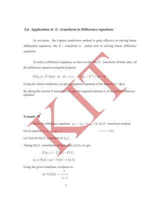
The inverse Z – transforms can be obtained by using any one of the following
methods.They are
I. Power series method
II. Partial fraction method
III. Inversion Integral method
IV. Long division method
5.4 Inverse Z – Transforms
K
IT](https://image.slidesharecdn.com/mechma6351tpdenotes1-180418083523/85/Mech-MA6351-tpde_notes-185-320.jpg)
![Now,
Z-1
{F(z). G (z)} = fn * gn = an
* bn
n
= am
bn-m
m=0
n a m
= bn
------- which is a G.P.
m=0
b
(a/b) n+1
- 1
= bn
-----------------------
(a/b) – 1
z2
an+1
– bn+1
ie, Z-1
---------------- = ---------------------
(z-a) (z-b) a–b
Example 17
z 3
Find z-1
-------- by using convolution theorem
(z-1)
z2
z
Let F (z) = ---------- and G (z) -----------
(z-1)2
(z-1)
Then fn = n+1 & gn = 1
By convolution Theorem, we have
n
Z-1
{ F(z). G (z) } = fn * gn = (n+1) * 1 = (m+1) . 1
m=0
(n+1) (n+2)
= --------------------
2
Example 18
Use convolution theorem to find the inverse Z- transform of
1
--------------------------------
[1 – (1/2)z –1
] [1- (1/4)z-1
]
K
IT](https://image.slidesharecdn.com/mechma6351tpdenotes1-180418083523/85/Mech-MA6351-tpde_notes-194-320.jpg)
![Given Z-1
------------------------------ - = Z-1
---------------------------
[1 – (1/2)z –1
] [1- (1/4)z-1
] [z-(1/2)] [z – (1/4)]
z z
Let F (z) = -------------- & G (z) = -------------
z – (1/2) z – (1/4)
Then fn = (1/2)n
& gn = (1/4)n
.
We know that Z-1
{ F(z). G(z)} = fn * gn
= (1/2)n
* (1/4)n
n 1 m
1 n - m
= ------- -------
m=0
2 4
1 n
n 1 m
1 -m
= ------ ------- -------
4 m=0
2 4
1 n
n
= ------ 2 m
4 m=0
1 n
= ------ { 1+2+22
+ . . . + 2n
} which is a G.P
4
1 n 2n+1
- 1
= ------ --------------
4 2-1
1 n
= ------ {2n+1
– 1}
4
1 1 n
= ---------- - -------
2n-1
4
1 1 1
Z-1
--------------------------------- = ------ - -------
[1 – (1/2)z –1
] [1- (1/4)z-1
] 2 n-1
4 n
1 z2
K
IT](https://image.slidesharecdn.com/mechma6351tpdenotes1-180418083523/85/Mech-MA6351-tpde_notes-195-320.jpg)
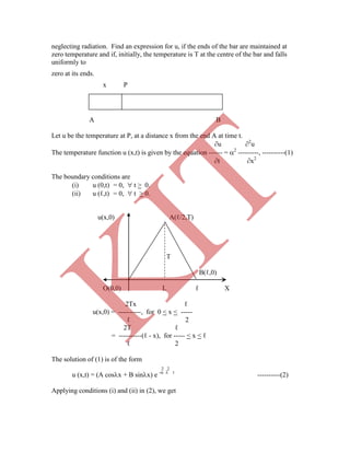
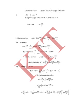
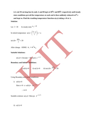
( aayaaxz ---------------(5)
Diff (5) p.w.r.to a, we get
x0
22
)]([12
)(')(22
)('
aa
aaa
ya
-----------------------(6)
Eliminate a between (5) abd (6) to get the general solution.
2.Solve y2
p-xyq=x(z-2y)
Soln:
Given y2
p-xyq=x(z-2y)
This equation of the form Pp+Qq=R
K
IT](https://image.slidesharecdn.com/mechma6351tpdenotes1-180418083523/85/Mech-MA6351-tpde_notes-212-320.jpg)
![Integrating, we get 0
111
dz
z
dy
y
dx
x
logx +logy+logz=log b
Hence the general solution is,
F(x2
+y2
+z2
, logx +logy+logz)=0.
5.Solve:[D3
-2D2
D’]z=ex+2y
+4sin (x+y)
Soln:
Given: [D3
-2D2
D’]z=ex+2y
+4sin (x+y)
The auxiliary equation is m3
-2m2
=0
Replace D by m and D’ by 1
m2
(m-2)=0
m=0,0 and m=2
C.F= )2()()( 321 xyyxy
2yx
2y+x
23
2y+x
231
e
3
1
2byD'and1byDReplace
e
)2(2(1)-(1)
1
e
D'2D-D
1
.
IP
K
IT](https://image.slidesharecdn.com/mechma6351tpdenotes1-180418083523/85/Mech-MA6351-tpde_notes-216-320.jpg)
![( ) cos ( )f x x x f x
( )f x is an odd function. Hence 0 0a .
19. Write the Fourier sine series of k in ,0 .
The Fourier sine series is given by
1
( ) sinn
n
f x b nx
where nb =
1
( )sin .f x nx dx
0
2
sink nxdx
0
2 cos 2
1 ( 1)nk nx k
n n
i.e.,
4
, if is even
0, if is odd
n
k
n
b n
n
is odd
4
( ) sin
n
k
f x nx
n
=
1
4 1
sin[(2 1) ]
(2 1)n
k
n x
n
.
20. Obtain the sine series for unity in (0, )π .
Here ;1xf
1
( ) sinn
n
f x b nx
where nb =
1
( )sin .f x nx dx
0
2
1.sin .nx dx
0
2 cos 2
1 ( 1)nnx
n n
i.e.,
4
, if is even
0, if is odd
n
n
b n
n
K
IT](https://image.slidesharecdn.com/mechma6351tpdenotes1-180418083523/85/Mech-MA6351-tpde_notes-223-320.jpg)
![
is odd
4
( ) sin
n
f x nx
n
=
1
4 1
sin[(2 1) ]
(2 1)n
n x
n
.
21. Find the value of na , in the cosine series expansion of f x k in the interval 0,10 .
10
0
2
cos
10 10
n
n x
a k dx
10
0
sin
1010 sin 0 0
5 5
10
n x
k k
n
n n
.
22. If f x is defined in 3 3x what is the value of Fourier coefficients.
3 3 3
0
3 3 3
1 1 1
; cos ; sin
3 3 3 3 3
n n
n x n x
a f x dx a f x dx b f x dx
.
23. Define Root Mean Square value of a function.
The root mean square value of ( )y f x in ( , )a b is denoted by y . It is defined as
2
R.M.S.,
( )
b
a
y dx
y
b a
.
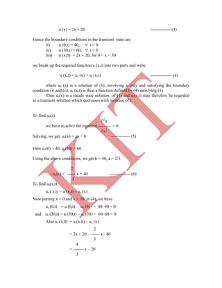
24. Find the R.M.S value of 2
,y x in .
K
IT](https://image.slidesharecdn.com/mechma6351tpdenotes1-180418083523/85/Mech-MA6351-tpde_notes-224-320.jpg)
![
5
22 2 5 51 1 1
2 2 5 10
x
y x dx
4 2
2
5 5
y y
.
25. Find the R.M.S value if 2
( )f x = x in π x π .
Since R.M.S
2
( )
b
a
y dx
y
b a
22
[ ( )]
x dx
4
2
x dx
5
4 4
0 0 0
2
5
2
x
x dx x dx
5
5
2
5
.
26. State the Parseval’s Identity (or) theorem on Fourier series.
If ( )f x is a periodic function of period 2 in ( , 2 )c c with Fourier coefficients
0, n na a and b , then
2 2
2 2 20
1
1
( )
2
c
n n
nc
a
f x dx a b .
27. Write the complex form of Fourier series for f(x) defined in the interval (c, c+2l).
The series for ( )f x defined in the interval ( , 2 )c c and satisfying Dirichlet’s
conditions can be given in the form of
K
IT](https://image.slidesharecdn.com/mechma6351tpdenotes1-180418083523/85/Mech-MA6351-tpde_notes-225-320.jpg)
![
33
2)1(2
2
n
l
n
l
l
k n
]1)1([2
2
3
n
n
l
l
k
= 33
2
4
n
kl
n
11
=
evenn
oddn
n
kl
,0
,
8
33
2
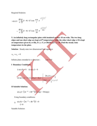
Required Solution:
y(x,t)=
5,3,1
33
2
8
n n
kl
sin
l
xn
cos
l
ctn
l
ctn
l
xn
n
kl
n
)12(
cos
)12(
sin
)12(
18
0
33
2
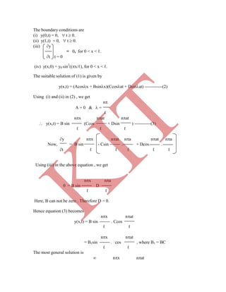
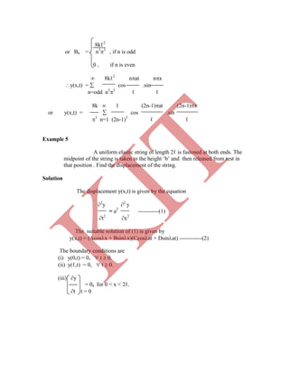
2.A taut string of length 2l is fastened at both ends . The midpoint of the string is taken to a
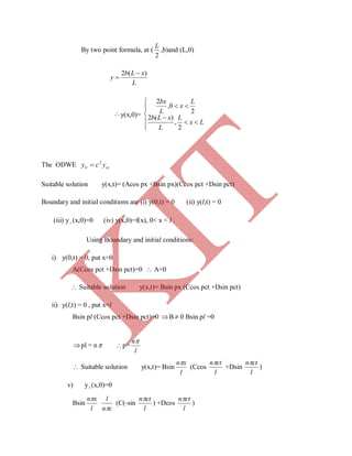
height b and then released from rest in that position. Find the displacement of the string at
any time.
Solution: let L=2l
Equation of AC: 2
0
L
x
By two point formula: at (0,0) and (
2
L
,b)
b
y
L
x
2/
L
bx
y
2
Equation of CB:
2
L
<x<L
K
IT](https://image.slidesharecdn.com/mechma6351tpdenotes1-180418083523/85/Mech-MA6351-tpde_notes-251-320.jpg)
![
2
2
s
F f x F s e .
10. Prove that
1
cos ( ) ( )
2
c c cF f x ax F s a F s a where cF denotes the Fourier
cosine
transform f x .
The F.C.T is,
0
2
( )cos
cF f x f x sxdx
0
2
cos ( )cos cos
cF f x ax f x ax sxdx
0
coscos)(
2
axdxsxxf
dxxasxasxf )cos()cos(
2
1
)(
2
0
0 0
)cos()(
2
)cos()(
2
2
1
xdxasxfxdxasxf
)]()([
2
1
asFcasFc .
11. Prove that
s
c
d F f x
F x f x
ds
.
W.k.t
0
2
( )sin
sF f x f x sxdx
K
IT](https://image.slidesharecdn.com/mechma6351tpdenotes1-180418083523/85/Mech-MA6351-tpde_notes-266-320.jpg)
![18. Find the Fourier Sine transform of f(x)= x
e
.
We know that
0
2
[ ( )] ( )sinsF f x f x sxdx
0
2
[ ] sin
x x
sF e e sxdx
2 2 2
0
2
sin ]
1
axs b
e bxdx
s a b
.
19. Find the Fourier Sine transform of x
e 2
3
.
Let 2
3 x
f x e
W.k.t
0
2
sinsF f x f x sxdx
dxsxe x
sin3
2
0
2
dxsxe x
sin
2
3
0
2
0
2
2
cossin2
4
2
3 sxssx
s
e x
s
s2
4
1
0
2
3
4
2
3 2
s
s
4
32
2
s
s
.
20. Find the Fourier Sine transform of
x
1
.
We know that
K
IT](https://image.slidesharecdn.com/mechma6351tpdenotes1-180418083523/85/Mech-MA6351-tpde_notes-270-320.jpg)
![Statement:
If F s and G s are the Fourier transform of f x and g x respectively. Then the
Fourier transforms of the convolution of f x and g x is the product of their Fourier
transforms.
*F f x g x F s G s
F f x F g x .
Where
dttxgtfxgf )()(
2
1
PROOF: By convolution of two functions:
dttxgtfxgf )()(
2
1
The Fourier transform of gf is
F[ gf ]
dxegf isx
)(
2
1
dxedttxgtf isx
)()({
2
1
2
1
dxetxgdttf isx
)()(
2
1
Put u=x-t du=dx x= u= and x=- u=-
F[ gf ]
dueugdttf tuis )(
)()(
2
1
dueugdtetf isuist
)(
2
1
)(
2
1
K
IT](https://image.slidesharecdn.com/mechma6351tpdenotes1-180418083523/85/Mech-MA6351-tpde_notes-272-320.jpg)
![F[( gf )(x)]=F(s)G(s)
2.Find the Fourier transform of
in,0
in,
)(
22
ax
axxa
xf
Hence evaluate
4
cossin
0
3
dt
t
ttt
Solution: Given:
in,0
in,
)(
22
ax
axxa
xf
F(s)
dxexf isx
)(
2
1
a
a
isx
dxexa )(
2
1 22
a
sxdxxa
0
22
cos)(
2
1
0
sin2cos2
2
2
32
s
as
s
asa
3
cossin
2
4
s
asasas
3
cossin2
2
s
asasas
3. Show that 2
2
x
e
is reciprocal with respect to Fourier transforms
Solution:
Fourier transform:
K
IT](https://image.slidesharecdn.com/mechma6351tpdenotes1-180418083523/85/Mech-MA6351-tpde_notes-273-320.jpg)
![F[f(x)] dxexf isx
)(
2
1
dxee isx
x
2
2
2
1
dxe
isx
x
2
2
2
1
dxee
sisx
22
)( 2
2
2
1
2
isx
y
dxdy
2
1
yx and yx
dyeesF
s
y
2
2
1
)( 2
2
2
dyee y
s
0
2
2
2
2
1
2
22
2
s
e
where
20
2
dye y
2
2
)(
s
esF
f(x)= 2
2
x
e
is self reciprocal with respect to Fourier transform.
4. Find the Fourier transform of
1if0
1if1
)(
x
xx
xf . Hence deduce that
3
sin
4
0
dt
t
t
Solution:
Fourier transform:
K
IT](https://image.slidesharecdn.com/mechma6351tpdenotes1-180418083523/85/Mech-MA6351-tpde_notes-274-320.jpg)
![F[f(x)] dxexf isx
)(
2
1
1
1
)1(
2
1
dxex isx
1
0
cos)1(
2
2
sxdxx
1
0
2
cos
)1(
sin
)1(
2
s
sx
s
sx
x
22
1cos2
ss
sx
2
cos12
)(
s
sx
sF
By parseval’s identity,
dxxfdssF
22
)()(
dxxf
2
)( =
1
1
2
1 dxx
1
0
2
12 dxx 1
0
3
1
3
2
x
1
0
3
1
3
2
x =
3
2
.
2
2
2 cos12
)(
s
s
sF
4
4
)2/(sin8
s
s
ds
s
s
dssF
4
4
2 )2/(sin8
)(
ds
s
s
0
4
4
)2/(sin16
Put t=s/2 2t=s 2dt=ds
tsts and00
dt
t
s
2
2
)2/(sin16
0
4
4
dt
t
t
0
4
4
sin2
K
IT](https://image.slidesharecdn.com/mechma6351tpdenotes1-180418083523/85/Mech-MA6351-tpde_notes-275-320.jpg)
2(cos
2
)]([ sxdxxsxdxxxfFc
2
1
2
1
0
2
cos
)1(
sin
)2(
cossin2
s
sx
s
sx
x
s
sx
s
sx
x
2222
cossin2cos1cossin2
s
s
s
s
s
s
ss
s
s
s
222
12coscos22
ss
s
s
s
6. Find the Fourier cosine transform of
22
xa
e
Solution:
0
cos)(
2
)]([ sxdxxfxfFc
0
cos
2
)]([
22
sxdxexfF xa
c
K
IT](https://image.slidesharecdn.com/mechma6351tpdenotes1-180418083523/85/Mech-MA6351-tpde_notes-276-320.jpg)
(
2
)]([ sxdxxfxfFs
22
2
as
s
By inversion formula,
0
sin)]([
2
)( sxdsxfFxf s
K
IT](https://image.slidesharecdn.com/mechma6351tpdenotes1-180418083523/85/Mech-MA6351-tpde_notes-277-320.jpg)
![)(sin
22
0
22
xfsxds
as
s
ax
exfsxds
as
s
2
)(
2
sin
0
22
,a>0
8. Evaluate
0
2222
bxax
dx
using Fourier Cosine Transform.
Solution:
22
2
][
as
a
eF ax
c
By Parseval’s identity
00
)()()()( dxxgxfdssGsF cc
00
2222
22
dxeeds
bs
b
as
a bxax
0
2222
)(
1
))((
2
babsas
dsab
put s=x
0
2222
)(
1
2))(( baabbxax
dx
9. Evaluate
0
22
)4)(1( xx
dx
Solution:
Proving
0
22
)(
1
2)4)(1( baabxx
dx
Put a=1 and b=2
12)3)(2)(1)(2()4)(1(0
22
xx
dx
K
IT](https://image.slidesharecdn.com/mechma6351tpdenotes1-180418083523/85/Mech-MA6351-tpde_notes-278-320.jpg)
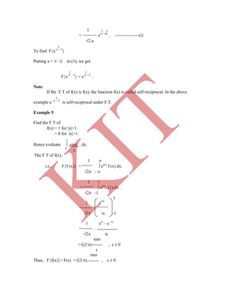
![10. Using Parseval’s identity evaluate:
0
222
2
ax
dxx
Solution;
Consider the function ax
exf
)(
22
2
][
as
s
eF ax
s
By parseval’s identity,
0
2
0
2
)]([)]([ dxxfdssFc
0
2
0
2
22
][
2
dxeds
as
s ax
0
2
0
222
2
2
2
a
e
ds
as
s ax
put s=x
aa
dx
ax
x
422
1
0
222
2
UNIT V
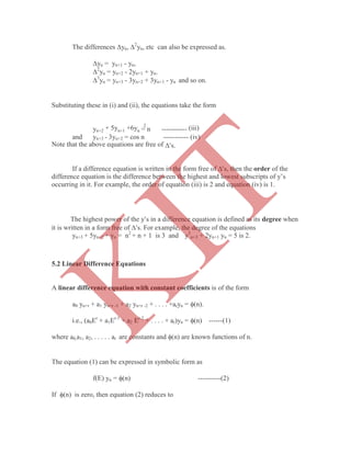
Z -TRANSFORMS AND DIFFERENCE EQUATIONS
PART – A
1. Prove that aZ
z
aZ n
is az .
We know that
0
n
n
Z x n x n z
K
IT](https://image.slidesharecdn.com/mechma6351tpdenotes1-180418083523/85/Mech-MA6351-tpde_notes-279-320.jpg)
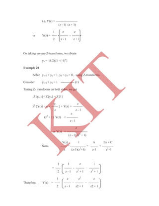
![PART B
1. Using the Z transforms, Solve
Solution:
Given
[
( ) U (z)- -2z-3z = 0 [ ]
U (z) =
U (z) =
= = + …………… (1)
Then
Put z = -1, we get Put z = -2, we get
4 =A 3 = -B
A = 4 B = -3
(1) = -[
U (z) = -3[
K
IT](https://image.slidesharecdn.com/mechma6351tpdenotes1-180418083523/85/Mech-MA6351-tpde_notes-289-320.jpg)
![Z [u(n)] = -3[
u(n) = -3 [
= 4( - 3(
= [4-3( )] (
2. Solve the difference equation
Solution:
Given
[
[ [ ]
[
[
[
Y (z) =
=
=
=
= ……….(1)
K
IT](https://image.slidesharecdn.com/mechma6351tpdenotes1-180418083523/85/Mech-MA6351-tpde_notes-290-320.jpg)
![Put z=1 , we get Put z =-2 , we get
8 = 3A -4 = -3B
A=8/3 B = 4/3
(1)
Z[y(n)] =
y(n) =
=
3. Using Z transforms, Solve ,
Solution:
Given
]
[
( ) U (z)-z = , ]
( ) U (z) = z+
=
=
=
K
IT](https://image.slidesharecdn.com/mechma6351tpdenotes1-180418083523/85/Mech-MA6351-tpde_notes-291-320.jpg)
![=
=
= = + …………… (1)
Put z = 2, we get Put z = 4, we get
1 =-2A 1= 2B
A = - B =
(2) = +[
U (z) = - +[
Z [u(n)] = - + [
u(n) = - [
= -
4.Using Z transforms, Solve ,
Solution:
Given
[
( ) Y (z) = ,
( ) Y (z) =
Y (z) =
K
IT](https://image.slidesharecdn.com/mechma6351tpdenotes1-180418083523/85/Mech-MA6351-tpde_notes-292-320.jpg)
This unit covers the formation and solutions of partial differential equations (PDEs). PDEs can be obtained by eliminating arbitrary constants or functions from relating equations. Standard methods are used to solve first order PDEs and higher order linear PDEs with constant coefficients. Various physical processes are modeled using PDEs including the wave equation, heat equation, and Laplace's equation.