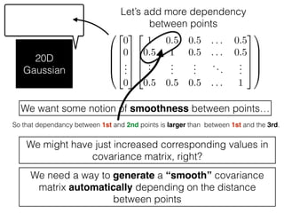
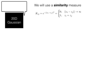
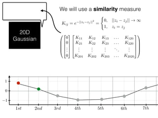
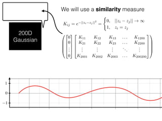
Download as PDF, PPTX


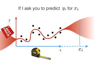

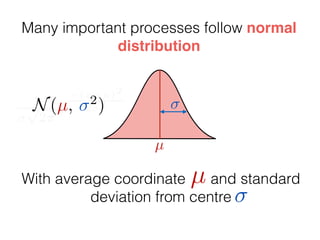


![What is ?
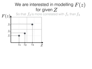
f1
f2
f3
Zz1 z2 z3
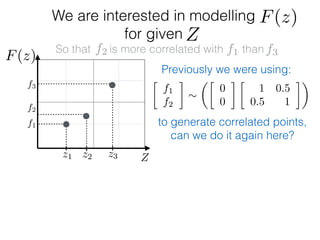
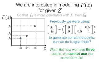
F(z)
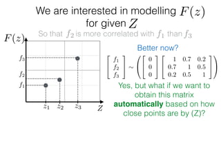
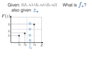
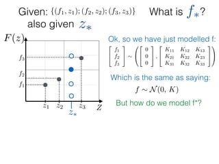
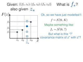
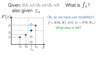
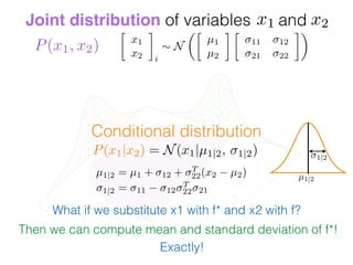
Given: {(f1, z1); (f2, z2); (f3, z3)}
z⇤
z⇤also given
f⇤
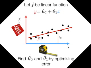
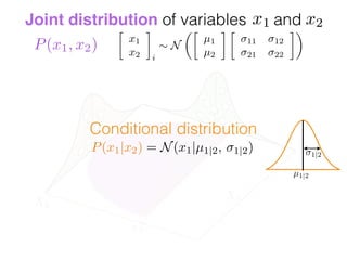
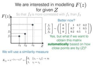
Ok, so we have just modelled f:
What else is left?
f ⇠ N(0, K) and f⇤ ⇠ N(0, K⇤⇤)
f
f⇤
⇠
0
B
B
B
B
@
0
0
2
6
6
6
6
4
2
4
K11 K12 K13
K21 K22 K23
K31 K32 K33
3
5
2
4
K1⇤
K2⇤
K3⇤
3
5
⇥
K⇤1 K⇤2 K⇤3
⇤
[K⇤⇤]
3
7
7
7
7
5
1
C
C
C
C
A](https://image.slidesharecdn.com/gp-181018124759/85/Introduction-to-Gaussian-Processes-118-320.jpg)
![What is ?
f1
f2
f3
Zz1 z2 z3
F(z)
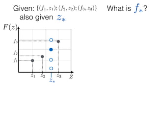
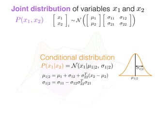
Given: {(f1, z1); (f2, z2); (f3, z3)}
z⇤
z⇤also given
f⇤
Ok, so we have just modelled f:
What else is left?
f ⇠ N(0, K) and f⇤ ⇠ N(0, K⇤⇤)
f
f⇤
⇠
0
B
B
B
B
@
0
0
2
6
6
6
6
4
2
4
K11 K12 K13
K21 K22 K23
K31 K32 K33
3
5
2
4
K1⇤
K2⇤
K3⇤
3
5
⇥
K⇤1 K⇤2 K⇤3
⇤
[K⇤⇤]
3
7
7
7
7
5
1
C
C
C
C
A
K
1](https://image.slidesharecdn.com/gp-181018124759/85/Introduction-to-Gaussian-Processes-119-320.jpg)
![What is ?
f1
f2
f3
Zz1 z2 z3
F(z)
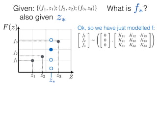
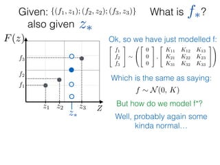
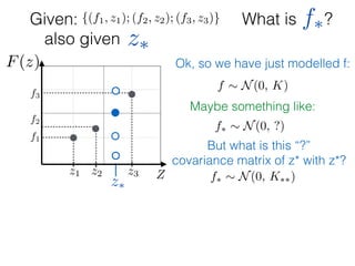
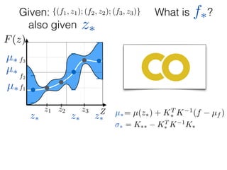
Given: {(f1, z1); (f2, z2); (f3, z3)}
z⇤
z⇤also given
f⇤
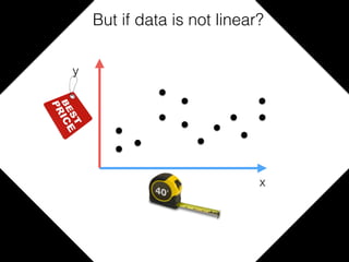
Ok, so we have just modelled f:
What else is left?
f ⇠ N(0, K) and f⇤ ⇠ N(0, K⇤⇤)
f
f⇤
⇠
0
B
B
B
B
@
0
0
2
6
6
6
6
4
2
4
K11 K12 K13
K21 K22 K23
K31 K32 K33
3
5
2
4
K1⇤
K2⇤
K3⇤
3
5
⇥
K⇤1 K⇤2 K⇤3
⇤
[K⇤⇤]
3
7
7
7
7
5
1
C
C
C
C
A
K
1
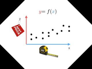
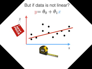
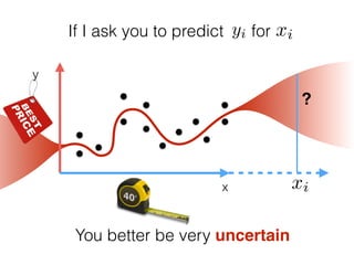
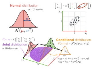
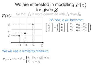
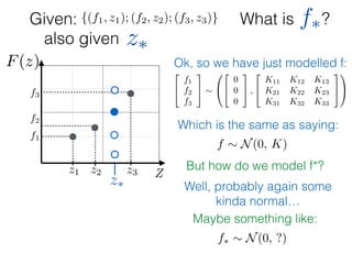
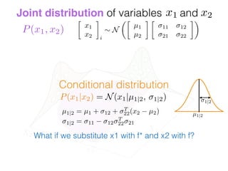
Only one entity is left:
K1⇤ = K(z1, z⇤)](https://image.slidesharecdn.com/gp-181018124759/85/Introduction-to-Gaussian-Processes-120-320.jpg)
![What is ?
f1
f2
f3
Zz1 z2 z3
F(z)
Given: {(f1, z1); (f2, z2); (f3, z3)}
z⇤
z⇤also given
f⇤
Ok, so we have just modelled f:
What else is left?
f ⇠ N(0, K) and f⇤ ⇠ N(0, K⇤⇤)
f
f⇤
⇠
0
B
B
B
B
@
0
0
2
6
6
6
6
4
2
4
K11 K12 K13
K21 K22 K23
K31 K32 K33
3
5
2
4
K1⇤
K2⇤
K3⇤
3
5
⇥
K⇤1 K⇤2 K⇤3
⇤
[K⇤⇤]
3
7
7
7
7
5
1
C
C
C
C
A
K
1
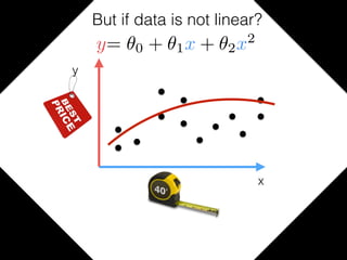
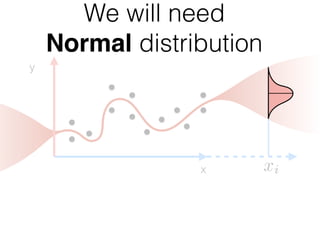
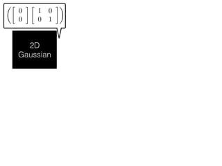
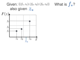
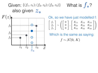
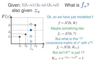
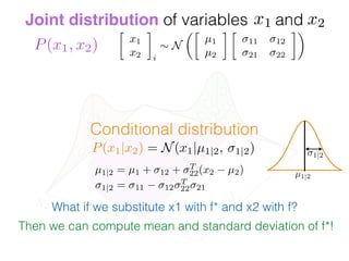
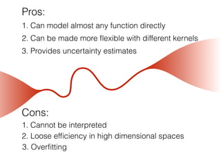
Only one entity is left:
K1⇤ = K(z1, z⇤)
I guess we know how to
calculate this one!
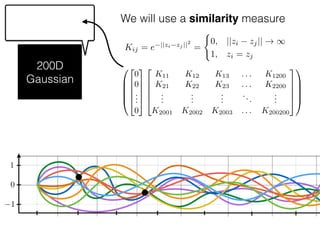
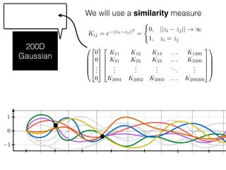
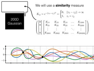
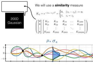
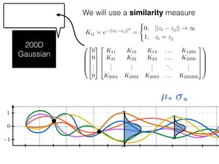
Kij = e ||zi zj ||2
=
(
0, ||zi zj|| ! 1
1, zi = zj](https://image.slidesharecdn.com/gp-181018124759/85/Introduction-to-Gaussian-Processes-121-320.jpg)
![What is ?
f1
f2
f3
Zz1 z2 z3
F(z)
Given: {(f1, z1); (f2, z2); (f3, z3)}
z⇤
z⇤also given
f⇤
Ok, so we have just modelled f:
f ⇠ N(0, K) and f⇤ ⇠ N(0, K⇤⇤)
f
f⇤
⇠
0
B
B
B
B
@
0
0
2
6
6
6
6
4
2
4
K11 K12 K13
K21 K22 K23
K31 K32 K33
3
5
2
4
K1⇤
K2⇤
K3⇤
3
5
⇥
K⇤1 K⇤2 K⇤3
⇤
[K⇤⇤]
3
7
7
7
7
5
1
C
C
C
C
A
K
1
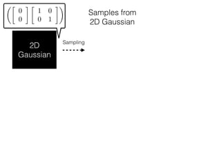
Ki⇤
K⇤i
Yeah! We did it!](https://image.slidesharecdn.com/gp-181018124759/85/Introduction-to-Gaussian-Processes-122-320.jpg)
![What is ?
f1
f2
f3
Zz1 z2 z3
F(z)
Given: {(f1, z1); (f2, z2); (f3, z3)}
z⇤
z⇤also given
f⇤
Ok, so we have just modelled f:
f ⇠ N(0, K) and f⇤ ⇠ N(0, K⇤⇤)
f
f⇤
⇠
0
B
B
B
B
@
0
0
2
6
6
6
6
4
2
4
K11 K12 K13
K21 K22 K23
K31 K32 K33
3
5
2
4
K1⇤
K2⇤
K3⇤
3
5
⇥
K⇤1 K⇤2 K⇤3
⇤
[K⇤⇤]
3
7
7
7
7
5
1
C
C
C
C
A
K
1
Ki⇤
K⇤i
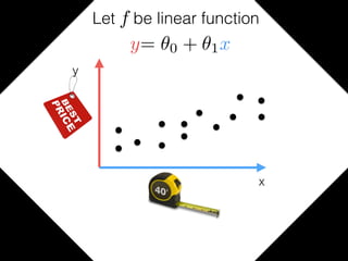
Yeah! We did it!
Wait… but what we do now?](https://image.slidesharecdn.com/gp-181018124759/85/Introduction-to-Gaussian-Processes-123-320.jpg)
![What is ?
f1
f2
f3
Zz1 z2 z3
F(z)
Given: {(f1, z1); (f2, z2); (f3, z3)}
z⇤
z⇤also given
f⇤
Ok, so we have just modelled f:
f ⇠ N(0, K) and f⇤ ⇠ N(0, K⇤⇤)
f
f⇤
⇠
0
B
B
B
B
@
0
0
2
6
6
6
6
4
2
4
K11 K12 K13
K21 K22 K23
K31 K32 K33
3
5
2
4
K1⇤
K2⇤
K3⇤
3
5
⇥
K⇤1 K⇤2 K⇤3
⇤
[K⇤⇤]
3
7
7
7
7
5
1
C
C
C
C
A
K
1
Ki⇤
K⇤i
Yeah! We did it!
Wait… but what we do now?
Remember….](https://image.slidesharecdn.com/gp-181018124759/85/Introduction-to-Gaussian-Processes-124-320.jpg)
![What is ?
f1
f2
f3
Zz1 z2 z3
F(z)
Given: {(f1, z1); (f2, z2); (f3, z3)}
z⇤
z⇤also given
f⇤
Ok, so we have just modelled f:
f ⇠ N(0, K) and f⇤ ⇠ N(0, K⇤⇤)
f
f⇤
⇠
0
B
B
B
B
@
0
0
2
6
6
6
6
4
2
4
K11 K12 K13
K21 K22 K23
K31 K32 K33
3
5
2
4
K1⇤
K2⇤
K3⇤
3
5
⇥
K⇤1 K⇤2 K⇤3
⇤
[K⇤⇤]
3
7
7
7
7
5
1
C
C
C
C
A
K
1
Ki⇤
K⇤i
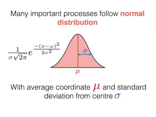
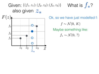
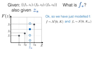
µ⇤= µ(z⇤) + KT
⇤ K 1
(f µf )](https://image.slidesharecdn.com/gp-181018124759/85/Introduction-to-Gaussian-Processes-129-320.jpg)
![What is ?
f1
f2
f3
Zz1 z2 z3
F(z)
Given: {(f1, z1); (f2, z2); (f3, z3)}
z⇤
z⇤also given
f⇤
Ok, so we have just modelled f:
f ⇠ N(0, K) and f⇤ ⇠ N(0, K⇤⇤)
f
f⇤
⇠
0
B
B
B
B
@
0
0
2
6
6
6
6
4
2
4
K11 K12 K13
K21 K22 K23
K31 K32 K33
3
5
2
4
K1⇤
K2⇤
K3⇤
3
5
⇥
K⇤1 K⇤2 K⇤3
⇤
[K⇤⇤]
3
7
7
7
7
5
1
C
C
C
C
A
K
1
Ki⇤
K⇤i
µ⇤
µ⇤= µ(z⇤) + KT
⇤ K 1
(f µf )](https://image.slidesharecdn.com/gp-181018124759/85/Introduction-to-Gaussian-Processes-130-320.jpg)
![What is ?
f1
f2
f3
Zz1 z2 z3
F(z)
Given: {(f1, z1); (f2, z2); (f3, z3)}
z⇤
z⇤also given
f⇤
Ok, so we have just modelled f:
f ⇠ N(0, K) and f⇤ ⇠ N(0, K⇤⇤)
f
f⇤
⇠
0
B
B
B
B
@
0
0
2
6
6
6
6
4
2
4
K11 K12 K13
K21 K22 K23
K31 K32 K33
3
5
2
4
K1⇤
K2⇤
K3⇤
3
5
⇥
K⇤1 K⇤2 K⇤3
⇤
[K⇤⇤]
3
7
7
7
7
5
1
C
C
C
C
A
K
1
Ki⇤
K⇤i
µ⇤ ⇤
µ⇤= µ(z⇤) + KT
⇤ K 1
(f µf )
⇤ = K⇤⇤ KT
⇤ K 1
K⇤](https://image.slidesharecdn.com/gp-181018124759/85/Introduction-to-Gaussian-Processes-131-320.jpg)
![What is ?
f1
f2
f3
Zz1 z2 z3
F(z)
Given: {(f1, z1); (f2, z2); (f3, z3)}
z⇤
z⇤also given
f⇤
Ok, so we have just modelled f:
f ⇠ N(0, K) and f⇤ ⇠ N(0, K⇤⇤)
f
f⇤
⇠
0
B
B
B
B
@
0
0
2
6
6
6
6
4
2
4
K11 K12 K13
K21 K22 K23
K31 K32 K33
3
5
2
4
K1⇤
K2⇤
K3⇤
3
5
⇥
K⇤1 K⇤2 K⇤3
⇤
[K⇤⇤]
3
7
7
7
7
5
1
C
C
C
C
A
K
1
Ki⇤
K⇤i
µ⇤
µ⇤= µ(z⇤) + KT
⇤ K 1
(f µf )
⇤ = K⇤⇤ KT
⇤ K 1
K⇤](https://image.slidesharecdn.com/gp-181018124759/85/Introduction-to-Gaussian-Processes-132-320.jpg)
![What is ?
f1
f2
f3
Zz1 z2 z3
F(z)
Given: {(f1, z1); (f2, z2); (f3, z3)}
z⇤
z⇤also given
f⇤
Ok, so we have just modelled f:
f ⇠ N(0, K) and f⇤ ⇠ N(0, K⇤⇤)
f
f⇤
⇠
0
B
B
B
B
@
0
0
2
6
6
6
6
4
2
4
K11 K12 K13
K21 K22 K23
K31 K32 K33
3
5
2
4
K1⇤
K2⇤
K3⇤
3
5
⇥
K⇤1 K⇤2 K⇤3
⇤
[K⇤⇤]
3
7
7
7
7
5
1
C
C
C
C
A
K
1
Ki⇤
K⇤i
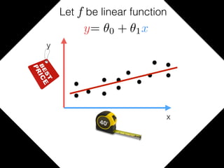
µ⇤
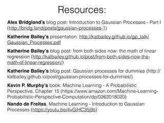
z⇤ z⇤
µ⇤
µ⇤
µ⇤= µ(z⇤) + KT
⇤ K 1
(f µf )
⇤ = K⇤⇤ KT
⇤ K 1
K⇤](https://image.slidesharecdn.com/gp-181018124759/85/Introduction-to-Gaussian-Processes-133-320.jpg)
![What is ?
f1
f2
f3
Zz1 z2 z3
F(z)
Given: {(f1, z1); (f2, z2); (f3, z3)}
z⇤
z⇤also given
f⇤
Ok, so we have just modelled f:
f ⇠ N(0, K) and f⇤ ⇠ N(0, K⇤⇤)
f
f⇤
⇠
0
B
B
B
B
@
0
0
2
6
6
6
6
4
2
4
K11 K12 K13
K21 K22 K23
K31 K32 K33
3
5
2
4
K1⇤
K2⇤
K3⇤
3
5
⇥
K⇤1 K⇤2 K⇤3
⇤
[K⇤⇤]
3
7
7
7
7
5
1
C
C
C
C
A
K
1
Ki⇤
K⇤i
µ⇤
z⇤ z⇤
µ⇤
µ⇤
µ⇤= µ(z⇤) + KT
⇤ K 1
(f µf )
⇤ = K⇤⇤ KT
⇤ K 1
K⇤](https://image.slidesharecdn.com/gp-181018124759/85/Introduction-to-Gaussian-Processes-134-320.jpg)
![What is ?
f1
f2
f3
Zz1 z2 z3
F(z)
Given: {(f1, z1); (f2, z2); (f3, z3)}
z⇤also given
f⇤
Ok, so we have just modelled f:
f ⇠ N(0, K) and f⇤ ⇠ N(0, K⇤⇤)
f
f⇤
⇠
0
B
B
B
B
@
0
0
2
6
6
6
6
4
2
4
K11 K12 K13
K21 K22 K23
K31 K32 K33
3
5
2
4
K1⇤
K2⇤
K3⇤
3
5
⇥
K⇤1 K⇤2 K⇤3
⇤
[K⇤⇤]
3
7
7
7
7
5
1
C
C
C
C
A
K
1
Ki⇤
K⇤i
µ⇤
µ⇤
µ⇤
z⇤z⇤ z⇤
µ⇤= µ(z⇤) + KT
⇤ K 1
(f µf )
⇤ = K⇤⇤ KT
⇤ K 1
K⇤](https://image.slidesharecdn.com/gp-181018124759/85/Introduction-to-Gaussian-Processes-135-320.jpg)


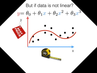
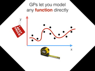
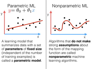
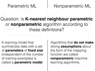
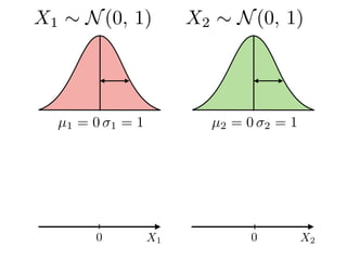
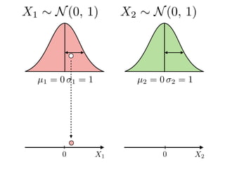
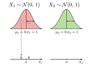
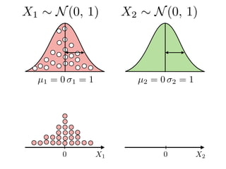
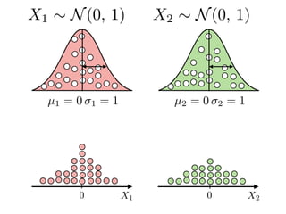
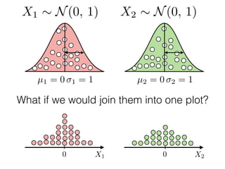
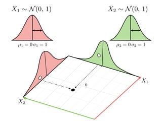
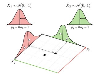
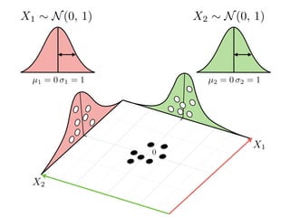
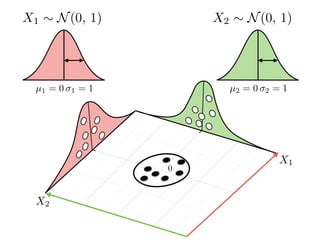
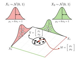
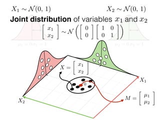
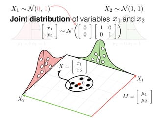
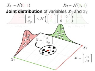
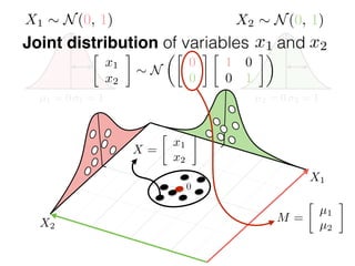
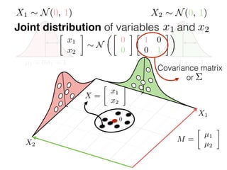
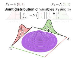
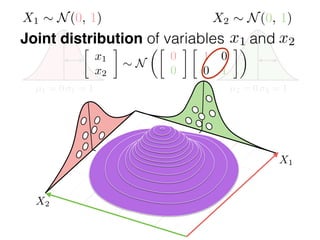
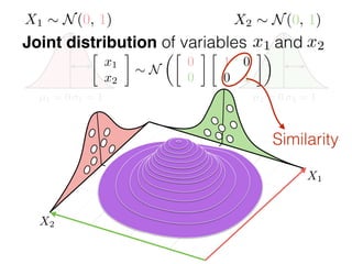
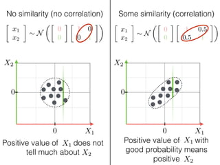
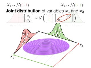
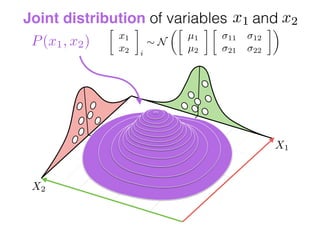
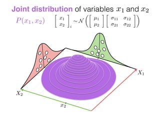
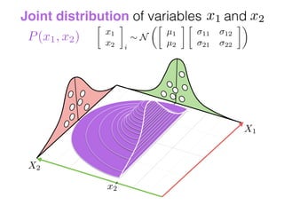
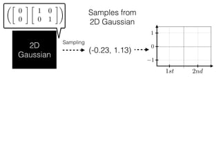
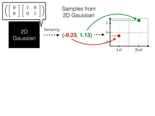
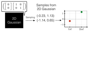
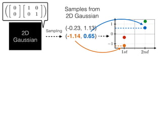
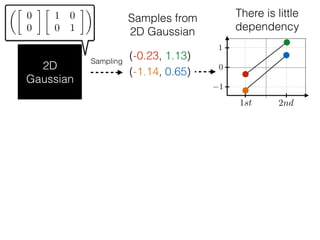
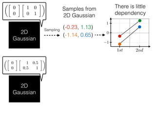
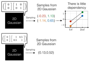
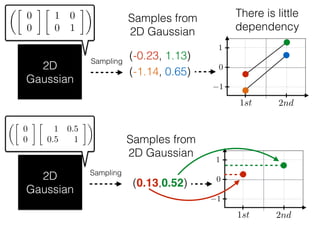
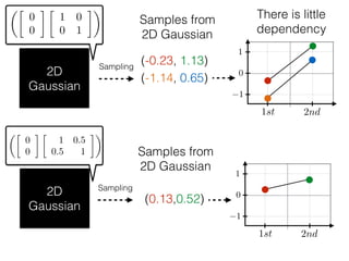
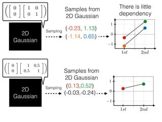
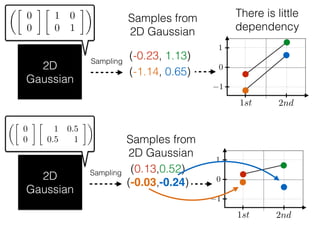
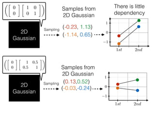
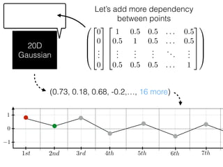
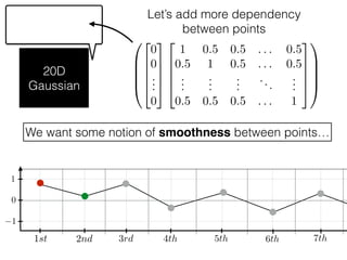
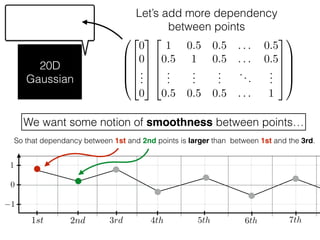
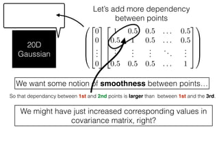
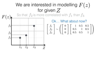
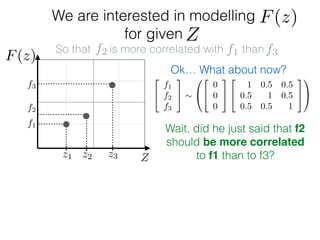
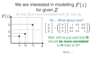
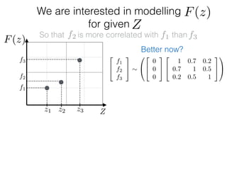
The document provides an introduction to Gaussian processes. It explains that Gaussian processes allow modeling any function directly and estimating uncertainty for predictions. It demonstrates how two random variables can be jointly distributed as a multivariate Gaussian distribution, and how the conditional distribution of one variable given the other can be derived from the joint distribution. Gaussian processes use these properties to perform nonparametric machine learning by modeling relationships between variables without assuming a specific function form.